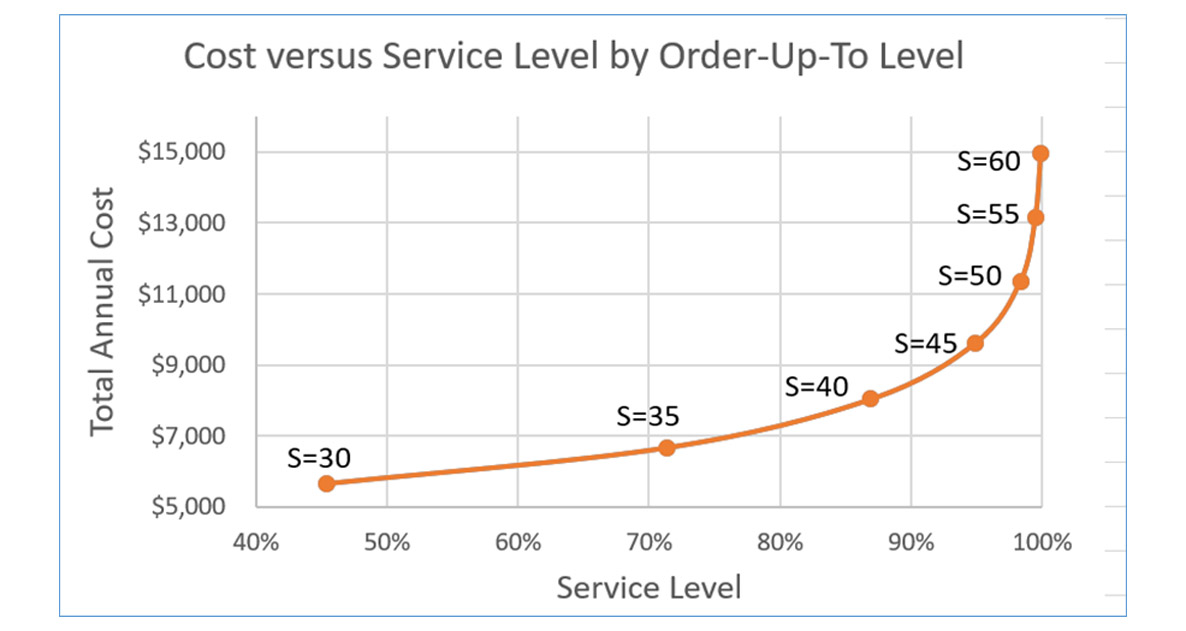
Those who produce forecasts owe it to those who consume forecasts, and to themselves, to be aware of the uncertainty in their forecasts. This note is about how to estimate forecast uncertainty and use the estimates in your demand planning process. We focus on forecasts made in support of demand planning as well as forecasts inherent in optimizing inventory policies involving reorder points, safety stocks, and min/max levels.

Reading this, you will learn about:

-Criteria for assessing forecasts
-Sources of forecast error
-Calculating forecast error
-Converting forecast error into prediction intervals
-The relationship between demand forecasting and inventory optimization.
-Actions you can take to use these concepts to improve your company’s processes.

Criteria for Assessing Forecasts

Forecast error alone is not reason enough to reject forecasting as a management tool. To twist a famous aphorism by George Box, “All forecasts are wrong, but some are useful.” Of course, business professionals will always search for ways to make forecasts more useful. This usually involves work to reduce forecast error. But while forecast accuracy is the most obvious criterion by which to judge forecasts, but it is not the only one. Here’s a list of criteria for evaluating forecasts:

Accuracy: Forecasts of future values should, in retrospect, be very close to the actual values that eventually reveal themselves. But there may be diminishing returns to squeezing another half percent of accuracy out of forecasts otherwise good enough to use in decision making.

Timeliness: Fighter pilots refer to the OODA Loop (Observe, Orient, Decide, and Act) and the “need to get inside the enemy’s OODA loop” so they can shoot first. Businesses too have decision cycles. Delivering a perfectly accurate forecast the day after it was needed is not helpful. Better is a good forecast that arrives in time to be useful.

Cost: Forecasting data, models, processes and people all cost money.  A less expensive forecast might be fueled by data that are readily available; more expensive would be a forecast that runs on data that have to be collected in a special process outside the scope of a firm’s information infrastructure.  A classic, off-the-shelf forecasting technique will be less costly to acquire, feed and exploit than a complex, custom, consultant-supplied method. Forecasts could be mass-produced by software overseen by a single analyst, or they might emerge from a collaborative process requiring time and effort from large groups of people, such as district sales managers, production teams, and others. Technically advanced forecasting techniques often require hiring staff with specialized technical expertise, such as a master’s degree in statistics, who tend to cost more than staff with less advanced training.

Credibility: Ultimately, some executive has to accept and act on each forecast. Executives have a tendency to distrust or ignore recommendations that they can neither understand nor explain to the next person above them in the hierarchy. For many, believing in a “black box” is too severe a test of faith, and they reject the black box’s forecasts in favor of something more transparent.

All that said, we will focus now on forecast accuracy and its evil twin, forecast error.

Sources of Forecast Error

Those seeking to reduce error can look in three places to find trouble:
1. The data that goes into a forecasting model
2. The model itself
3. The context of the forecasting exercise

There are several ways in which data problems can lead to forecast error.

Gross errors: Wrong data produce wrong forecasts. We have seen an instance in which computer records of product demand were wrong by a factor of two! Those involved spotted that problem immediately, but a less egregious situation can easily slip through to poison the forecasting process. In fact, just organizing, acquiring and checking data is often the largest source of delay in the implementation of forecasting software. Many data problems seem to derive from the data having been unimportant until a forecasting project made them important.

Anomalies: Even with perfectly curated forecasting databases, there are often “needle in a haystack” type data problems. In these cases, it is not data errors but demand anomalies that contribute to forecast error. In a set of, say, 50,000 products, some number of items are likely to have odd details that can distort forecasts.

Holdout analysis is a simple but powerful method of analysis. To see how well a method forecasts, use it with older known data to forecast newer data, then see how it would have turned out! For instance, suppose you have 36 months of demand data and need to forecast 3 months ahead. You can simulate the forecasting process by holding out (i.e., hiding) the most recent 3 months of data, forecasting using only data from months 1 to 33, then comparing the forecasts for months 34-36 against the actual values in months 34-36. Sliding simulation merely repeats the holdout analysis, sliding along the demand history. The example above used the first 33 months of data to get 3 estimates of forecast error. Suppose we start the process by using the first 12 months to forecast the next 3. Then we slide forward and use the first 13 months to forecast the next 3. We continue until finally we use the first 35 months to forecast the last month, giving us one more estimate of the error we make when forecasting one month ahead. Summarizing all the 1-step ahead, 2-step ahead and 3-step ahead forecast errors provides a way to calculate prediction intervals.

Calculating Prediction Intervals

The final step in calculating prediction intervals is to convert the estimates of average absolute error into the upper and lower limits of the prediction interval. The prediction interval at any future time is computed as

Prediction interval = Forecast ± Multiplier x Average absolute error.

The final step is the choice of the multiplier. The typical approach is to imagine some probability distribution of error around the forecast, then estimate the ends of the prediction interval using appropriate percentiles of that distribution. Usually, the assumed distribution of error is the Normal distribution, also called the Gaussian distribution or the “bell-shaped curve”.

Use of Prediction Intervals
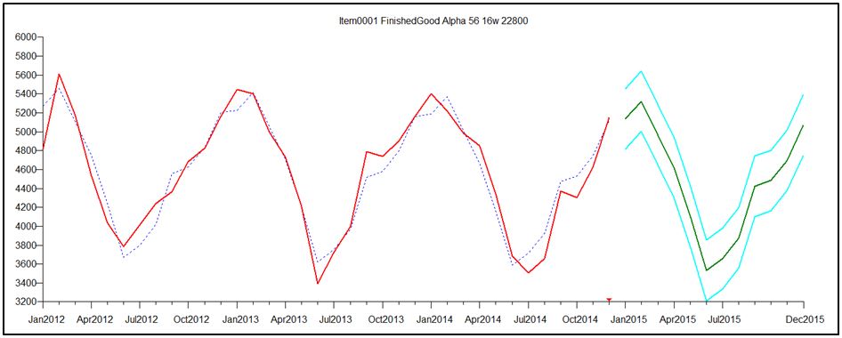
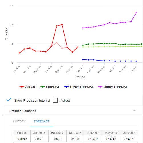
The most immediate, informal use of prediction intervals is to convey a sense of how “squishy” a forecast is. Prediction intervals that are wide compared to the size of the forecasts indicate high uncertainty.

There are two more formal uses in demand forecasting: Hedging your bets about future demand and guiding forecast adjustment.

Hedging your bets: The forecast values themselves approximate the most likely values of future demand. A more ominous way to say the same thing is that there is about a 50% chance that the actual value will be above (or below) the forecast. If the forecast is being used to plan future production (or raw materials purchase or hiring), you might want to build in a cushion to keep from being caught short if demand spikes (assuming that under-building is worse than over-building). If the forecast is converted from units to dollars for revenue projections, you might want to use a value below the forecast to be conservative in projecting cash flow. In either case, you first have to choose the coverage of the prediction interval. A 90% prediction interval is a range of values that covers 90% of the possibilities. This implies that there is a 5% chance of a value falling above the upper limit of the 90% prediction interval. In other words, the upper limit of a 90% prediction interval marks the 95th percentile of the distribution of predicted demand at that time period. Similarly, there is a 5% chance of falling below the lower limit, which marks the 5th percentile of the demand distribution.

Guiding forecast adjustment: It is quite common for statistical forecasts to be revised by some sort of collaborative process. These adjustments are based on information not recorded in an item’s demand history, such as intelligence about competitor actions. Sometimes they are based on a more vaporous source, such as sales force optimism. When the adjustments are made on-screen for all to see, the prediction intervals provide a useful reference: If someone wants to move the forecasts outside the prediction intervals, they are crossing a fact-based line and should have a good story to justify their argument that things will be really different in the future.

Prediction Intervals and Inventory Optimization

Finally, the concept behind prediction intervals play an essential role in a problem related to demand forecasting: Inventory Optimization.
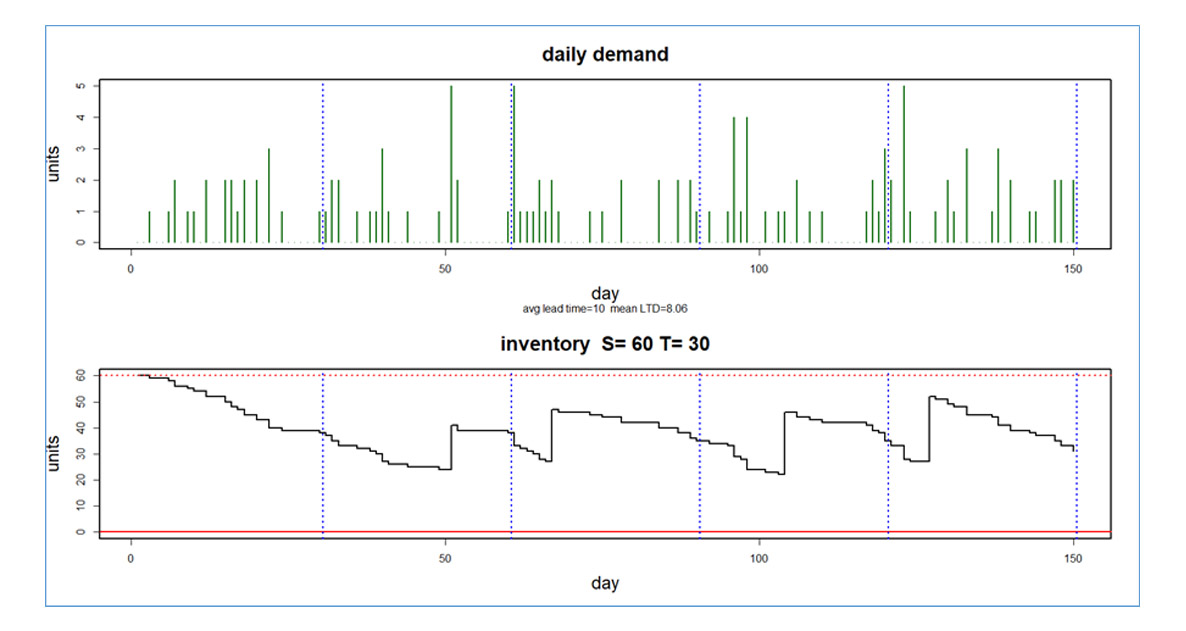
The core analytic task in setting reorder points (also called Mins) is to forecast total demand over a replenishment lead time. This total is called the lead time demand. When on-hand inventory falls down to or below the reorder point, a replenishment order is triggered. If the reorder point is high enough, there will be an acceptably small risk of a stockout, i.e., of lead time demand driving inventory below zero and creating either lost sales or backorders.

New statistical methods, and we can start planning more effectively.

The forecasting task is to determine all the possible values of cumulative demand over the lead time and their associated probabilities of occurring. In other words, the basic task is to determine a prediction interval for some future random variable. Suppose you have computed a 90% prediction interval for lead time demand. Then the upper end of the interval represents the 95th percentile of the distribution. Setting the reorder point at this level will accommodate 95% of the possible lead time demand values, meaning there will be only a 5% chance of stocking out before replenishment arrives to re-stock the shelves. Thus there is an intimate relationship between prediction intervals in demand forecasting and calculation of reorder points in inventory optimization.

5 Recommendations for Practice

1. Set expectations about error: Sometimes  managers have unreasonable expectations about reducing forecast error to zero. You can point out that error is only one of the dimensions on which a forecasting process must be judged; you may be doing fine on both timeliness and cost. Also point out that zero error is no more realistic a goal than 100% conversion of prospects into customers, perfect supplier performance, or zero stock price volatility.

2. Track down sources of error: Double check the accuracy of demand histories. Use statistical methods to identify outliers in demand histories and react appropriately, replacing verified anomalies with more typical values and omitting data from before major changes in the character of the demand. If you use a collaborative forecasting process, compare its accuracy against a purely statistical approach to identify items for which collaboration does not reduce error.

3. Evaluate the error of alternative statistical methods: There may be off-the-shelf techniques that do better than your current methods, or do better for some subsets of your items. The key is to be empirical, using the idea of holdout analysis. Gather your data and do a “bake off” between different methods to see which work better for you. If you are not already using statistical forecasting methods, compare them against whoever’s “golden gut” is your current standard. Use the naïve forecast as a benchmark in the comparisons.

4. Investigate the use of new data sources: Especially if you have items that are heavily promoted, test out statistical methods that incorporate promotional data into the forecasting process. Also check whether information from outside your company can be exploited; for instance, see whether macroeconomic indicators for your sector can be combined with company data to improve forecast accuracy (this is usually done using a method called multiple regression analysis).

5. Use prediction intervals: Plots of prediction intervals can improve your feel for the uncertainty in your forecasts, helping you select items for additional scrutiny. While it’s true that what you don’t know can hurt you, it’s also true that knowing what you don’t know can help you.

Improve Forecast Accuracy, Eliminate Excess Inventory, & Maximize Service Levels

In this Video Dr. Thomas Willemain, co–Founder and SVP Research, defines and compares the most useful Forecasting Techniques: Exponential Smoothing, Single Exponential Smoothing, Holt’s Method and Winter’s Method.  These videos explain the basic thinking under each technique as well as the math behind them, how they are used in practice and the tradeoff of each method.

In a previous post, I discussed one of the thornier problems demand planners sometimes face: working with product demand data characterized by what statisticians call skewness — a situation that can necessitate costly inventory investments. This sort of problematic data is found in several different scenarios. In at least one, the combination of intermittent demand and very effective sales promotions, the problem lends itself to an effective solution.

Reviewing terms, recall that “service level” is the probability of not stocking out while waiting for a replenishment order to arrive, while “fill rate” is the percentage of demand that is satisfied immediately from stock. In my previous post, “The Scourge of Skewness”, I pointed out that a certain type of demand distribution, having a “long right tail”, will lead to fill rates that can be much lower than service levels. I also pointed out that sometimes the only way to improve the fill rate is to increase the target service level to an unusually high level, which can be expensive.

In this post, I’ll look at solving the problem in one special case: skewness resulting from effective sales promotions mixed with “intermittent demand”. Intermittent demand has a large proportion of zero values, with nonzero values mixed in at random. Successful sales promotions, obviously positive, have a downside: they can confuse the “demand signal” with spikes in your demand history, and can undermine forecasts and bias safety stock calculations. When intermittent demand and effective sales promotions are the source of your data’s skewness, methods exist to work around the problem to achieve both higher fill rates and more accurate demand forecasts.

How Promotions Increase Skewness

Successful promotions abruptly increase item demand. This creates anomalies, or “outliers”, which contribute to forming a skewed distribution. Knowing when promotions occurred in the past, we can adjust an item’s record of past demand. We produce an alternate demand history as if there had been no promotions, by replacing the outliers with values more representative of the “natural” level of demand. These adjustments reduce demand skewness. Reduced skewness can lead to significant reductions in both expected forecasts and safety stocks, which add together to form reorder points.

Successful promotions are likely to be repeated. When that happens, the promotion effects can be added in to demand forecasts to increase their accuracy. The effect of future promotions on inventory management will be to increase the risk of stockouts, so a sensible response is to work at the operational level to build up temporary supply, in a quantity keyed to the estimated impact of prior promotions on the effected items.

Using Event Modeling to Improve Demand Forecasting

It’s possible to model the impact of like events, and apply this to planned events in the future. Doing so can improve your forecast in two big ways: by projecting the demand jolt you expect from a planned event; and rationalizing the spikes in the past that were caused by events, making your baseline activity more visible and more accurately forecastable. We do a lot of this in SmartForecasts, so allow me to use our experience there to show you what I mean.

Event Modeling entails the following steps:
• Automatically estimating the impact of previous promotions (which is a useful result in itself).
• Adjusting historical demand to statistically remove the effect of promotions.
• Creating promotion-free forecasts.
• Revising the forecasts for any future time periods in which promotions are planned.

We call this this type of analysis “Promo forecasting”. We use the word “promotions” to describe what you do yourself to improve your results. We use “events” to describe what the world does to you, usually to your detriment; examples include strikes, power outages, warehouse fires and other unlucky happenings.

To understand how Event Modeling can help you cope with skewness when doing demand forecasting for high-volume items, consider Figures 1-3.

Figure 1 shows that this item’s demand pattern is clearly seasonal, and the forecast is both seasonal and “tight”, meaning that the forecast uncertainty interval (“margin of error”, shown in cyan lines) is very narrow.

Figure 2 shows an alternative history in which a promotion in June 2014 reversed the usual seasonal low associated with June sales. This demand pattern was forecasted using the Automatic forecasting tournament in SmartForecasts, as in Figure 1. This time, the promotion scrambled the seasonal pattern enough to create an inappropriate non-seasonal forecast, and one that has a much larger margin of error.

Finally, Figure 3 shows how Promo forecasting handles the same promoted scenario, retaining a seasonal forecast and building into the forecast an estimate of the effect of a planned repeat promotion in 2015.

The Case of Intermittent Demand

In Figure 1, the item was a high-volume finished good and the task was demand forecasting. Promo modeling is also useful when dealing with the task of setting safety stocks and reorder points for items with intermittent demand, whether the items are finished goods, components or spare parts. Intermittent demand very often has a skewed distribution that makes it difficult to achieve high item availability with a small investment in inventory.

Figure 4 illustrates the problem that a successful promotion can accidentally create for inventory management. If such a spike arises from the natural, un-promoted demand, then the only way to maintain high fill rates is to provide safety stocks large enough to cope with these random surges. In this case, the big spike in demand of 500 units in February 2013 was the result of a one-time promotion.

Taking Account of Promotions to Improve Inventory Management

Unwittingly treating the spike in the example above as part of the natural demand variability results in a poor fill rate. To achieve a target service level of, say, 95% with a lead time of one month would require a reorder point of 38 units, computed as the sum of an expected forecast over the one month replenishment lead time of 21 units supplemented by a safety stock of 17 units. This investment would result in a disappointing fill rate of only 36%.

However, recognizing that the spike is a one-time promotion and replacing the 500 units with 0 obviously would make a big difference. The reorder point would drop from 38 units to 31 (the sum of an expected demand of 7 units and a safety stock of 24 units) and the fill rate would increase to 94%.

Of course, it is not ok to just throw out inconvenient demand spikes whenever they make life uncomfortable; there has to be a valid “business story” behind the adjustment of historical demand. If the spike is the result of a data processing error, then by all means, fix it. If the spike coincides with a promotion, then replacing the spike with, say, the median demand (often zero, as in this example) will result in a much more sustainable inventory investment that still meets aggressive performance targets. Future promotions of the same type on the same item will require some extra effort to prepare for the temporary surge in demand, but the recommended reorder point will be correct in the long run.

Thomas Willemain, PhD, co-founded Smart Software and currently serves as Senior Vice President for Research. Dr. Willemain also serves as Professor Emeritus of Industrial and Systems Engineering at Rensselear Polytechnic Institute and as a member of the research staff at the Center for Computing Sciences, Institute for Defense Analyses.

Anybody doing the job knows that managing inventory can be stressful. Common stressors include: Customers with “special” requests, IT departments with other priorities, balky ERP systems running on inaccurate data, raw material shortages, suppliers with long lead times in far-away countries where production often stops for various reasons and more. This note will address one particular and ever-present source of stress: demand variability.

Everybody Has a Forecasting Problem

Suppose you manage a large fleet of spare parts. These might be surgical equipment for your hospital, or repair parts for your power station. Your mission is to maximize up time. Your enemy is down time. But because breakdowns hit at random, you are constantly in reactive mode. You might hope for rescue from forecasting technologies. But forecasts are inevitably imperfect to some degree: the element of surprise is always present.  You might wait for Internet of Things (IOT) tech to be deployed on your equipment to monitor and detect impending failures, helping you schedule repairs well in advance. But you know you can’t meter up the thousands of small things that can fail and disable a big thing.

So, you decide to combine forecasting with inventory management and build buffers or safety stock to protect against surprise spikes in demand. Now you have to work out how much safety stock to maintain, knowing that too little means vulnerability and too much means bloat.

Suppose you handle finished goods inventories for a make-to-stock company. Your problem is essentially the same as in managing service parts: You have external customers and uncertain demand. But you may also have additional problems in terms of synchronizing multiple suppliers of components that you assemble into finished goods. The suppliers want you to tell them how much of their stuff to make so you can make your stuff, but you don’t know how much of your own stuff you’ll need to make.

Finally, suppose you handle finished goods in a build-to-order company. You might think that you no longer have a forecasting problem, since you don’t build until you are paid to build. But you do have a forecasting problem. Since your finished goods might be assembled from a mixture of components and sub-assemblies, you have to translate some forecast of finished goods demand to work out a forecast of those components. Otherwise, you will go to make your finished goods and discover that you don’t have a required component and have to wait until you can re-actively assemble everything you need. And your customers might not be willing to wait.

So, everybody has a forecasting problem.

What Makes Forecasting Difficult

Forecasting can be quick, easy and dead accurate – as long as the world is simple. If demand for your product is 10 units every week, month after month, you can make very accurate forecasts. But life is not quite like that. If you’re lucky and life is almost like that – maybe weekly demand is more like {10, 9, 10, 8, 12, 10, 10…} — you can still make very accurate forecast and just make minor adjustments around the edges. But if life is as it more often is – maybe weekly demand looks like {0, 0, 7, 0, 0, 0, 23, 0 …} – demand forecasting is difficult indeed. The key distinction is demand variability: it’s the zigging and zagging that creates the pain.

Safety Stock Takes Over Where Forecasting Leaves Off

Statistical forecasting methods are an important part of the solution. They let you squeeze as much advantage as possible from the historical patterns of demand your company has recorded for each item. The job of forecasts is to describe what is typical, which provides the base on which to cope with randomness in demand. Statistical forecasting techniques work by finding “big picture” features in demand records, such as trend and seasonality, then projecting those into the future. They all implicitly assume that whatever patterns exist now will persist, so 5% growth will continue, and July demand will always be 20% higher than February demand. To get to that point, statistical forecasting methods use some form of averaging to smother the “noise” in the demand history.

But then the rest of the job falls on inventory management, because the atypical, random component of future demand will still be a hassle in the future. This inevitable level of uncertainty has to be handled by the “shock-absorber” called safety stock.

The same methods that produce forecasts of trend and/or seasonality can be used to estimate the amount of forecast error. This has to be done carefully using a method called “holdout analysis”.  It works like this. Suppose you have 365 observations of daily demand for Item X, which has a replenishment lead time of 10 days. You want to know how many units will be demanded over some future 10-day period. You might input the first 305 days of demand history into the forecasting technique and get forecasts for the next 10 days, days 306-315.

The answer gives you one estimate of the 10-day total demand. Importantly, it also gives you one estimate of the variability around that forecast, i.e., the forecast error, the difference between what actually happened in days 306-315 and what was forecasted. Now you can repeat the process, this time using the first 306 days to forecast the next 10, the first 307 days to forecast the next 10, etc. You end up with 52 honest estimates of the variability of total demand over a 10-day lead time. Suppose 95% of those estimates are less than 28 units. Then 28 units would be a pretty safe safety stock to add to the forecast, since you will run into shortages only 5% of the time.

Modern statistical software does these calculations automatically. It can ease at least one of the chronic headaches of inventory management by helping you cope with demand variability.

In another blog we posed the question:  How can you be sure that you really have a policy for inventory planning and demand forecasting? We explained how an organization’s lack of understanding on the basics (how a forecast is created, how safety stock buffers are determined, and how/why these values are adjusted) contributes to poor forecast accuracy, misallocated inventory, and lack of trust in the whole process.

In this blog, we review 10 specific questions you can ask to uncover what’s really happening at your company. We detail the typical answers provided when a forecasting/inventory planning policy doesn’t really exist, explain how to interpret these answers, and offer some clear advice on what to do about it.

Always start with a simple hypothetical example. Focusing on a specific problem you just experienced is bound to provoke defensive answers that hide the full story. The goal is to uncover the actual approach used to plan inventory and forecasts that has been baked into the mental math or spreadsheets.   Here is an example:

Suppose you have 100 units on hand, the lead time to replenish is 3 months, and the average monthly demand is 20 units?   When should you order more?  How much would you order? How will your answer change if expected receipts of 10 per month were scheduled to arrive?  How will your answer change if the item is the item is an A, B, or C item, the cost of the item is high or low, lead time of the item is long or short?  Simply put, when you schedule a production job or place a new order with a supplier, why did you do it? What triggered the decision to get more?  What planning inputs were considered?

When getting answers to the above question, focus on uncovering answers to the following questions:

1. What is the underlying replenishment approach? This will typically be one of Min/Max, forecast/safety stock, Reorder Point/Order Quantity, Periodic Review/Order Up To or even some odd combination

2. How are the planning parameters, such as demand forecasts, reorder points, or Min/Max, actually calculated? It’s not enough to know that you use Min/Max.  You have to know exactly how these values are calculated. Answers such as “We use history” or “We use an average” are not specific enough.   You’ll need answers that clearly outline how history is used.  For example, “We take an average of the last 6 months, divide that by 30 to get a daily average, and then multiply that by the lead time in days.  For ‘A’ items we then multiply the lead time average by 2 and for ‘B’ items we use a multiplier of 1.5.” (While that is not an especially good technical approach, at least it has a clear logic.)

Once you have a policy well-defined, you can identify its weaknesses in order to improve it.  But if the answer provided doesn’t get much further past “We use history”, then you don’t have a policy to start with.   Answers will often reveal that different planners use history in different ways.  Some may only consider the most recent demand, others might stock according to the average of the highest demand periods, etc.  In other words, you may find that you actually have multiple ill-conceived “policies”.

3. Are forecasts used to drive replenishment planning and if so, how? Many companies will say they forecast, but their forecasts are calculated and used differently. Is the forecast used to predict what on hand inventory will be in the future, resulting in an order being triggered?  Or is it used to derive a reorder point but not to predict when to order (i.e. I predict we’ll sell 10 a week so to help protect against stock out, I’ll order more when on hand gets to 15)? Is it used as a guide for the planner to help subjectively determine when they should order more?  Is it used to set up blanket orders with suppliers?  Some use it to drive MRP. You’ll need to know these specifics.  A thorough answer to this question might look like this: “My forecast is 10 per week and my lead time is 3 weeks so I make my reorder point a multiple of that forecast, typically 2 x lead time demand or 60 unit for important items and I use a smaller multiple for less important items.  (Again, not a great technical approach, but clear.)

4.  What technique is actually used to generate the forecast? Is it an average, a trending model such as double exponential smoothing, a seasonal model? Does the choice of technique change depend on the type of demand data or when new demand data is available? (Spare parts and high-volume items have very different demand patterns.) How do you go about selecting the forecast model? Is this process automated?  How often is the choice of model reconsidered?  How often are the model parameters recomputed? What is the process used to reconsider your approach?  The answer here documents how the baseline forecasts are produced.  Once determined, you can conduct an analysis to identify whether other forecasting methods would improve forecast accuracy.  If you aren’t documenting forecast accuracy and conducting “forecast value add” analysis then you aren’t in a position to properly assess whether the forecasts being produced are the best that they can be.  You’ll miss out on opportunities to improve the process, increase forecast accuracy, and educate the business on what type of forecast error is normal and should be expected.

5. How do you use safety stock? Notice the question was not “Do you use safety stock?” In this context, and to keep it simple, the term “safety stock” means stock used to buffer inventory against supply and demand variability.  All companies use buffering approaches in some way.  There are some exceptions though.  Maybe you are a job shop manufacturer that procures all parts to order and your customers are completely fine waiting weeks or months for you to source material, manufacture, QA, and ship.  Or maybe you are high-volume manufacturer with tons of buying power so your suppliers set up local warehouses that are stocked full and ready to provide inventory to you almost immediately.  If these descriptions don’t describe your company, you will definitely have some sort of buffer to protect against demand and supply variability.  You may not use the “safety stock” field in your ERP but you are definitely buffering.

Answers might be provided such as “We don’t use safety stock because we forecast.”  Unfortunately, a good forecast will have a 50/50 chance of being over/under the actual demand.  This means you’ll incur a stock out 50% of the time without a safety stock buffer added to the forecast.  Forecasts are only perfect when there is no randomness. Since there is always randomness, you’ll need to buffer if you don’t want to have abysmal service levels.

If the answer isn’t revealed, you can probe a bit more into how the varying replenishment levers are used to add possible buffers which leads to questions 6 & 7.

6. Do you ever increase the lead time or order earlier than you truly need to?
In our hypothetical example, your supplier typically takes 4 weeks to deliver and is pretty consistent. But to protect against stockouts your buyer routinely orders 6 weeks out instead of 4 weeks.  The safety stock field in your ERP system might be set to zero because “we don’t use safety stock”, but in reality, the buyer’s ordering approach just added 2 weeks of buffer stock.

7. Do you pad the demand forecast?
In our example, the planner expects to consume 10 units per month but “just in case” enters a forecast of 20 per month.  The safety stock field in the MRP system is left blank but the now disguised buffer stock has been smuggled into the demand forecast.  This is a mistake that introduces “forecast bias.”  Not only will your forecasts be less accurate but if the bias isn’t accounted for and safety stock is added by other departments, you will overstock.

The ad-hoc nature of the above approaches compounds the problems by not considering the actual demand or supply variability of the item. For example, the planner might simply make a rule of thumb that doubles the lead time forecast for important items.  One-size doesn’t fit all when it comes to inventory management.  This approach will substantially overstock the predictable items while substantially understocking the intermittently demanded items. You can read “Beware of Simple Rules of Thumb for Managing Inventory” to learn more about why this type of approach is so costly.

The ad-hoc nature of the approaches also ignores what happens the company is faced with a huge overstock or stock out. When trying to understand what happened, the stated policies will be examined. In the case of an overstock, the system will show zero safety stock.  The business leaders will assume they aren’t carrying any safety stock, scratch their heads, and eventually just blame the forecast, declare “Our business can’t be forecasted” and stumble on. They may even blame the supplier for shipping too early and making them hold more than needed. In the case of a stock out, they will think they aren’t carrying enough and arbitrarily add more stock across many items not realizing there is in fact lots of extra safety stock baked into process.  This makes it more likely inventory will need to be written off in the future.

8. What is the exact inventory terminology used? Define what you mean by safety stock, Min, reorder point, EOQ, etc.  While there are standard technical definitions it’s possible that something differs, and miscommunication here will be problematic.  For example, some companies refer to Min as the amount of inventory needed to satisfy lead time demand while some may define Min as inclusive of both lead time demand and safety stock to buffer against demand variability. Others may mean the minimum order quantity.

9. Is on hand inventory consistent with the policy? When your detective work is done and everything is documented, open your spreadsheet or ERP system and look at the on-hand quantity. It should be more or less in line with your planning parameters (i.e. if Min/Max is 20/40 and typical lead time demand is 10, then you should have roughly 10 to 40 units on hand at any given point in time.  Surprisingly, for many companies there is often a huge inconsistency. We have observed situations where the Min/Max setting is 20/40 but the on-hand inventory is 300+.  This indicates that whatever policy has been prescribed just isn’t being followed.   That’s a bigger problem.

10. What are you going to do next?

Demand forecasting and inventory stocking policy need to be well-defined processes that are understood and accepted by everybody involved.  There should be zero mystery.

To do this right, the demand and supply variability must be analyzed and used to compute the proper levels of safety stock.   Adding buffers without an implicit understanding of what each additional unit of buffer stock is buying you in terms of service is like arbitrarily throwing a handful of ingredients into a cake recipe.  A small change in ingredients can have a huge impact on what comes out of the oven – one bite too sweet but the next too sour.  It is the same with inventory management.  A little extra here, a little less there, and pretty soon you find yourself with costly excess inventory in some areas, painful shortages in others, no idea how you got there, and with little guidance on how to make things better.

Modern inventory optimization and demand planning software with its advanced analytics and strong basis in forecast analysis can help a good deal with this problem. But even the best software won’t help if it is used inconsistently.

What We’re Up Against

As a third-generation Boston Red Sox fan, I’m disinclined to take advice from any New York Yankee ballplayer, even a great one but have to agree that sometimes, you just need to make a decision.   However, wouldn’t it be better if we knew the tradeoffs associated with each decision. Perhaps one road is more scenic but takes longer while the other is more direct but boring. Then you wouldn’t have to simply “take it” but could make an informed decision based on the advantages/disadvantages of each approach.

In the supply chain planning world, the most fundamental decision is how to balance item availability against the cost of maintaining that availability (service levels and fill rates). At one extreme, you can grossly overstock and never run out until you go broke and have to close up shop from sinking all your cash into inventory that doesn’t sell.  At the other extreme, you can grossly understock and save a bundle on inventory holding costs but go broke and have to close up shop because all your customers took their business elsewhere.

There is no escaping this fundamental tension. They way to survive and thrive is to find a productive and sustainable balance. To do that requires fact-based tradeoffs based on the numbers. To get the numbers requires software.

The general drift of things is obvious. If you decide to keep more inventory, you will have more Holding Costs, lower Shortage Costs, and possibly lower Ordering Costs. Whether this costs or saves money is impossible to know without some sophisticated analysis, but usually the result is that the Total Cost goes up. But if you do invest in more inventory, something will be gained, because you will offer your customers higher Service Levels and Fill Rates. How much higher requires, as you might guess, some sophisticated analysis.

Show Me the Numbers

This blog lays out what such an analysis looks like. There is no universal solution pointing you to the “right” decision. You might think that the right decision is the one that does best by your bottom line. But to get those numbers, you would need something rarely seen: an accurate model of customer behavior with regard to service level (check out our article “How to choose a target service level”) For example, at what point will a customer walk away and take their business elsewhere?  Will it be after you stock out 1% of the time, 5% of time, 10% of the time? Will you still keep their business as long as you fill back orders quickly?  Will it be after a back order of 1 day, 2 days? 3 weeks? Will it be after this happens one time on one an important part or many times across many parts?  While modeling the precise service level that will allow you to keep your customer while minimizing costs seems like an unapproachable ideal, another type of sophisticated analysis is more pragmatic. 

Inventory optimization and forecasting software can factor all associated costs such as the cost of stocking out, cost of holding inventory, and cost of ordering inventory in order to prescribe an optimal service level target that yields the lowest total cost. However, even that “optimal” service level is sensitive to changes in the costs making the results potentially questionable.  For example, if you don’t accurately estimate the precise costs (shortage costs are the most difficult) it will be tough to definitely state something like “If I increase my on-hand inventory by an average of one unit for all items in an important product family, my company will see a net gain of $170,500.  That gain increases until I get to 4 units.  At 4 units and higher, the return declines due to excessive holding costs. So, the best decision factoring projected holding, ordering, and stockout is to increase inventory by 3 units to see a net gain of over $500,000.  

Short of that ideal, you can do something that is simpler yet still extremely valuable: Quantify the tradeoff curve between inventory cost and item availability. While you won’t necessarily know the service level you should target, you will know the costs of varying service levels.  Then you can earn your big bucks by finding a good place to be on that tradeoff curve and communicating where you at risk, where you aren’t, and setting expectations with customers and internal stakeholders.  Without the tradeoff curve to guide you, you are flying blind with no way to rationally modify stocking policy.

A Scenario to Learn From

Let’s sketch out a realistic tradeoff curve. We start with a scenario requiring a management decision. The scenario we will use and associated assumptions about demand, lead times, and costs are detailed below:

Inventory Policy

• Periodic review – Reorder decisions made every 30 days
• Order-Up-To-Level (“S”) – Varied from 30 to 60 units
• Shortage Policy – Allow backorders, no lost orders

Demand

• Demand is intermittent
• Average = 0.8 units per day
• Standard deviation = 1.2 units per day
• Largest demand in a year ≈ 9
• % of days with no demand = 53%

Lead Time

• Random at either 7, 14 or 21 days with probabilities 70%, 20% and 10%, respectively

Cost Parameters

• Holding cost = $1 per day
• Ordering Cost = $10 per order without regard to size of order
• Shortage Cost = $100 per unit not immediately shipped from stock

We imagine an inventory control policy that is known in the trade as a “periodic review” or (T,S) policy. In this instance, the Review Period (“T”) is 30 days, meaning that every 30 days the inventory position is checked and an ordering decision is made. The order quantity is the difference between the observed number of units on hand and the Order-Up-To Quantity (“S”). So, if the end-of-month inventory is 12 units and S = 20, the order quantity would be S – 12 = 20 -1 2 = 8. The next month, the order quantity is likely to be different. If the inventory ever goes negative (backorders) during a review period, the next order tries to restore equilibrium by ordering more in order to fill those backorders. For example, if the inventory is -5 (meaning 5 units ordered by not available for shipping, the next order would be S – (-5) = S + 5. Details of the hypothetical demand stream, supplier lead times, and cost elements are shown in Figure 1 below. Figure 2 show a sample of daily demand and daily inventory over five review periods. Demand is intermittent, as is often true for spare parts, and therefore difficult to plan for.

Figure 1: Different choices of inventory policy (order up to), associated costs, and service levels

Figure 2: Details of five months of system operation given one of the polices

Inventory Planning Software Is Our Friend

Software encodes the logic of the operation of the (T,S) system, generates many hypothetical but realistic demand scenarios, calculates how each of those scenarios plays out, then looks back on the simulated operation (here, 10 years or 3,650 consecutive days) to calculate cost and performance metrics.

To reveal the tradeoff curve, we ran several computational experiments in which we varied the Order-Up-To Level, S. The plots Figure 2 show the behavior of the on-hand inventory in “richest” alternative with S = 60. In the snippet shown in Figure 2, the on-hand inventory never comes close to stocking out. You can read that too ways. One, a bit naïve, is to say “Good, we’re well protected.” The other, more aggressive, is to say, “Oh no, we’re bloated. I wonder what would happen if we reduced S.”

The Tradeoff Curve Revealed

Figure 3 shows the results of reducing S from 60 down to 30 in steps of 5 units. The table shows that Total Cost is the sum of Holding Cost, Ordering Cost, and Shortage Cost. For the (T,S) policy, the ordering cost is always the same, since an order is placed like clockwork every 30 days. But the other components of cost respond to the changes in S.

Figure 3: The experimental results and corresponding tradeoff curve showing how changing the Order-Up-To Level (“S”) impacts both Service Level and Total Annual Cost

Note that the Service Level is always lower than the Fill Rate in these scenarios. As a professor, I always think of this difference in terms of exam grading. Each replenishment cycle is like a test. Service Level is about the probability of a stockout, so it’s a like the grade on pass/fail exam with one question that must be answered perfectly. If there is no stockout in a cycle, that’s an A. If there is a stockout, that’s an F. It doesn’t matter if it’s one unit that’s not supplied or 50 – it’s still an F. But Fill Rate is like a question that is graded with partial credit. So being short one of ten units gets you 90% Fill Rate for that cycle, not 0%. It’s important to understand the difference between these two important metrics for inventory planning – check out this vlog describing service level vs. fill rate via an interactive exercise in Excel.

The plot in Figure 3 is the real news. It pairs Total Cost and Service Level for various levels of S. If you read the graph right to left, it tells us that there are dramatic cost savings to be had by reducing S with very little penalty in terms of reduced item availability. For instance, reducing S from 60 to 55 saves close to $800 per year on this one item while reducing service level just a bit from (essentially) 100% to a still-impressive 99%. Cutting S some more does the same, though not as dramatically. If you read the graph left to right, you see that moving up from S = 30 to S = 35 costs about $1,000 per year but improves Service Level from an F grade (45%) to at least a C grade (71%). After that, pushing S higher costs progressively more while gaining progressive less.

The tradeoff curve doesn’t give you an answer to how to set the Order-Up-To Level, but it does let you evaluate the costs and benefits of each possible answer. Take a minute and pretend that this is your problem: Where would you want to be along the tradeoff curve?

You may object and say you hate your choices and want to change the game. Is there escape from the curve? Not from the general curve, but you might be able to shape a less painful curve. How?

You may have other cards to play. One avenue is to try to “shape” the demand so that it is less variable. The demand plot in Figure 2 shows a lot of variability. If you could smooth out the demand, the whole tradeoff curve would shift down, making every choice less expensive. A second avenue is to try to reduce the mean and variability of supplier lead times. Achieving either would also shift the curve down to make the choice less painful. Check out our article on how suppliers influence your inventory costs

Summary

The tradeoff curve is always with us. Sometimes we may be able to make it more friendly, but we always to pick our spot along it. It is better to know what you’re getting for any choice of inventory policy than to try to guess, and the curve gives you that.  When you have an accurate estimate of that curve, you are no longer flying blind when it comes to inventory planning.