
Software for inventory optimization is most often used to crank out the analytical results you need to run your day-to-day business, such as Reorder Points (also known as Mins) and Order Quantities. This specialized software helps you find the sweet spot that balances inventory costs against item availability during routine operations.
Inventory optimization software can also be used to perform “what-if” analyses on scenarios that describe changes from your current operating environment. What-if analysis (also called “sensitivity analysis”) lets you elevate your thinking from the tactical to the strategic. It helps you imagine how you should change your operations to adapt to potential changes in your operating environment. These changes might be negative pressures imposed on you from the outside, or they might result from your own positive actions. In this blog, we provide an example of how to conduct “what-analysis” on lead times and order quantities. Outputs from the analysis can be used by the business to assess the impact of these changes on inventory costs and service level performance.
How Suppliers Limit Your Freedom of Maneuver
Discussing with our customers the data inputs required by inventory optimization software, we noted that suppliers are a prominent influence on their operations. We leave aside for now such important topics as sharing demand forecasts with suppliers and working out responses to supply chain disruptions, such as Hurricane Matthew last year in the southeastern US. Instead, we focus on two more common ways that suppliers influence producers’ inventory costs: replenishment lead times and restrictions on order quantities.
Replenishment lead time is the number of days that elapse between inventory reaching or breaching a reorder point and the appearance of replenishment units in stock. Some portion of lead time is internal to the producer, perhaps due to slow reactions in a purchasing department. The rest of lead time is down to the supplier. In this discussion, we assume that suppliers’ contribution to lead times might be changed, for better or for worse. (But the same results could apply to changes in producers’ contributions to lead times.)
The restrictions on order quantities that we consider are order minima and order multiples. You might want to order 3 units of some item, but the supplier might impose a minimum order size of 6 units, so your 3 unit order would have to become a 6 unit order. Or you might want to order 21 units, handily exceeding the minimum order size of 6 units, but if the supplier also has an order multiple of 6, meaning every order must be a multiple of 6 units, then your 21 unit order would have to be increased to 24 units.
Scenario Analyses
To illustrate the use of inventory optimization software for what-if analysis, we examine two sets of scenarios. In the first set, lead times are varied from -20% to +20% of their values in a baseline scenario. In the second set, results are computed first with no supplier restrictions, then with order minima only, and finally with a combination of order minima and order multiples. We use Smart Inventory Optimization software for the calculations.
The baseline scenario uses real-world data on 2,852 spare parts managed by a progressive public transit agency. These parts have an extremely heterogeneous mix of attributes. Their per unit costs range from $1 to $23,105, and their lead times vary between 1 day and 300 days. Over 24 months, the mean demand ranged from less than 1 unit per month to 1,508 units per month, with coefficients of variation ranging from a manageable 10% to a scary 2,171%. Furthermore, the supplier picture is also very complex, involving 293 unique vendors, supplying an average of about 10 parts each. This heterogeneity implies that a real-world optimization would pick and choose among items and vendors. However, for simplicity of exposition and to develop basic insights, our what-if scenarios in this example treat every item and vendor equally. Similarly, we assumed in the baseline that holding costs equaled 20% of the dollar value of an item and that every replenishment order had a fixed cost of $40.
We conducted two what-if experiments. The first examined the effects of changing lead times. The second examined the effects of introducing restrictions on order quantities. In each experiment, we recorded the effects of the changes on two operational metrics: average number of units in stock and average number of orders per year. In turn, these influenced four financial metrics: average dollar value of inventory, average holding cost, average ordering cost, and the sum of the last two, which is total inventory operating cost.
In all scenarios, reorder points were calculated so as to achieve 95% probability of avoiding stockouts while waiting for replenishment. Order quantities, in the absence of supplier restrictions, were computed as what we call “feasible EOQ”. EOQ is the classic “economic order quantity” taught in Inventory 101; it is computed from average demand, holding cost and ordering cost. Feasible EOQ adds an additional consideration: inventory dynamics. If the reorder point is very low, it is possible for EOQ to be too small to sustain a stable, positive level of inventory. In these cases, feasible EOQ increases the order quantity above the EOQ to insure that average inventory does not go negative.
Effects of Changing Lead Times
Table 1 shows the results of changing the lead times. Working around the base case, we changed every item’s lead time by -20%, -10%, +10% and +20%.
It is no surprise that reducing lead times reduced the required level of inventory and increasing them did the opposite. Both the average number of units and the associated dollar value behaved as expected. What may be surprising is that the effects were somewhat muted, i.e., an X percent change in lead time produced a less-than-X percent response. For instance, a 20% reduction in lead time produced only a 7.9% reduction in on-hand inventory and only a 12.0% reduction in the dollar value of those units. Furthermore, the effects of reductions and increases are asymmetric: a 20% increase in lead time led to just a 7.3% increase in units (vs 7.9%) and only a 9.6% increase in inventory value (vs 12.0%).
Similar attenuated and asymmetric results held for operating costs. A 20% reduction in lead time decreased total operating costs by 7.0%, but a 20% increase in lead time caused only a 5.1% increase in operating costs.
Now consider the implications of these results for practice. In a competitive world, cost reductions on the order of 10% or even 5% are significant. This means that efforts to reduce lead times can have important payoffs. In turn, this means that efforts to streamline purchasing processes may be worth doing. Likewise, there is a case for engaging suppliers about reducing their part of lead time, possibly by sharing the savings to incentive them.
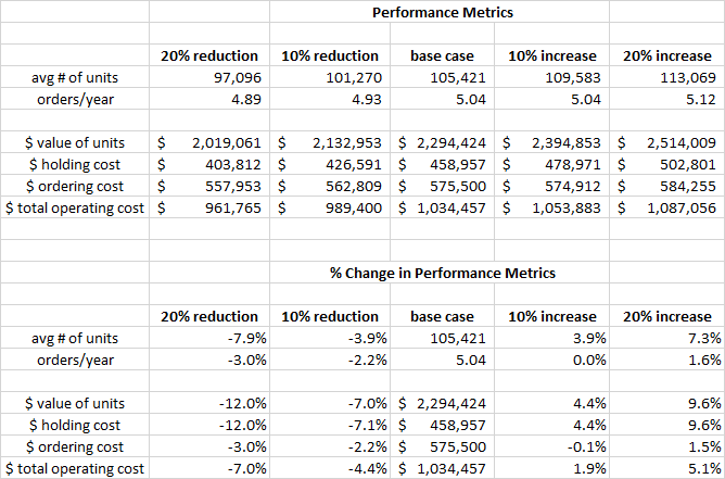
Table 1: Effects of changing lead times
Effect of Order Quantity Restrictions
Table 2 shows the effect of imposing supplier restrictions on order quantities. In the base case, there are no restrictions, i.e., the order minimum is 0 and the order multiple is 1, implying that any order quantity is acceptable to suppliers. Working away from the base case, we first looked at imposing an order minimum of 5 units on all items, then adding an order multiple of 5 for all items.
Forcing orders to be larger than they otherwise would be had the expected impact on the average number of units on hand, increasing it by 0.9% with only an order minimum and by 3.4% with both a minimum and a multiple. The corresponding changes in the dollar value of the inventory were more dramatic: 22.4% and 23.3%. This difference in the size of the percentage response probably traces back to the large number of low-volume/high-cost replacement parts managed by the public transit agency.
Another surprise was the net reduction in operating costs when supplier restrictions were imposed. While holding costs went up by 22.4% and 23.3% in the two what-if scenarios, the larger order quantities allowed for fewer orders per year, resulting in offsetting reductions in ordering costs of, respectively, -24.4% and -32.7%. The net impacts on operating costs were then reductions of 3.7% and 7.9%.
In general, placing restrictions on producer actions would be expected to reduce performance. So the results in these scenarios were counter-intuitive. However, the real message here is that using EOQ, or even enhanced EOQ, to set an order quantity does not give optimum results. Paradoxically, the order quantity restrictions we investigated seem to have forced order quantities closer to optimal levels.
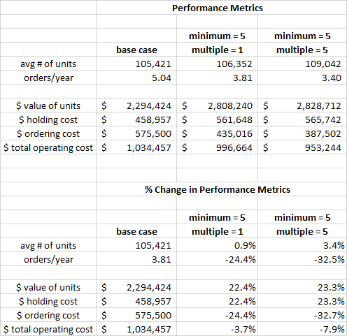
Table 2: Effect of order quantity restrictions
Conclusions
The what-if analyses shown here do not lead to universal conclusions. For instance, changing the assumed cost per order from $40 to some smaller number could show that the supplier restrictions increased rather than decreased the producer’s inventory operating costs.
When doing what-if analysis in real-word situations, users would naturally craft scenarios at a lower level of detail. For instance, they might evaluate the effect of changes in supplier lead times on a supplier-by-supplier basis to find the ones that would have the highest potential payoffs. Or they might arrange for order minima, if they exist already for all items, to change by a specified percentage instead of a fixed amount, which might be somewhat more realistic.
The key takeaway is that inventory optimization software can be used in “what-if mode” to explore strategic issues, beyond its customary use to calculate reorder points, safety stocks, order quantities, and inventory transfers.

Related Posts

Make AI-Driven Inventory Optimization an Ally for Your Organization
In this blog, we will explore how organizations can achieve exceptional efficiency and accuracy with AI-driven inventory optimization. Traditional inventory management methods often fall short due to their reactive nature and reliance on manual processes. Maintaining optimal inventory levels is fundamental for meeting customer demand while minimizing costs. The introduction of AI-driven inventory optimization can significantly reduce the burden of manual processes, providing relief to supply chain managers from tedious tasks.

Daily Demand Scenarios
In this Videoblog, we will explain how time series forecasting has emerged as a pivotal tool, particularly at the daily level, which Smart Software has been pioneering since its inception over forty years ago. The evolution of business practices from annual to more refined temporal increments like monthly and now daily data analysis illustrates a significant shift in operational strategies.

Constructive Play with Digital Twins
Those of you who track hot topics will be familiar with the term “digital twin.” Those who have been too busy with work may want to read on and catch up. While there are several definitions of digital twin, here’s one that works well: A digital twin is a dynamic virtual copy of a physical asset, process, system, or environment that looks like and behaves identically to its real-world counterpart. A digital twin ingests data and replicates processes so you can predict possible performance outcomes and issues that the real-world product might undergo.
Recent Posts
 Forecast-Based Inventory Management for Better PlanningForecast-based inventory management, or MRP (Material Requirements Planning) logic, is a forward-planning method that helps businesses meet demand without overstocking or understocking. By anticipating demand and adjusting inventory levels, it maintains a balance between meeting customer needs and minimizing excess inventory costs. This approach optimizes operations, reduces waste, and enhances customer satisfaction. […]
 Make AI-Driven Inventory Optimization an Ally for Your OrganizationIn this blog, we will explore how organizations can achieve exceptional efficiency and accuracy with AI-driven inventory optimization. Traditional inventory management methods often fall short due to their reactive nature and reliance on manual processes. Maintaining optimal inventory levels is fundamental for meeting customer demand while minimizing costs. The introduction of AI-driven inventory optimization can significantly reduce the burden of manual processes, providing relief to supply chain managers from tedious tasks. […]
 The Importance of Clear Service Level Definitions in Inventory ManagementInventory optimization software that supports what-if analysis will expose the tradeoff of stockouts vs. excess costs of varying service level targets. But first it is important to identify how “service levels” is interpreted, measured, and reported. This will avoid miscommunication and the false sense of security that can develop when less stringent definitions are used. Clearly defining how service level is calculated puts all stakeholders on the same page. This facilitates better decision-making. […]
 Future-Proofing Utilities: Advanced Analytics for Supply Chain OptimizationUtilities in the electrical, natural gas, urban water, and telecommunications fields are all asset-intensive and reliant on physical infrastructure that must be properly maintained, updated, and upgraded over time. Maximizing asset uptime and the reliability of physical infrastructure demands effective inventory management, spare parts forecasting, and supplier management. A utility that executes these processes effectively will outperform its peers, provide better returns for its investors and higher service levels for its customers, while reducing its environmental impact. […]
 The Cost of Spreadsheet PlanningCompanies that depend on spreadsheets for demand planning, forecasting, and inventory management are often constrained by the spreadsheet’s inherent limitations. This post examines the drawbacks of traditional inventory management approaches caused by spreadsheets and their associated costs, contrasting these with the significant benefits gained from embracing state-of-the-art planning technologies. […]

Inventory Optimization for Manufacturers, Distributors, and MRO
- Future-Proofing Utilities: Advanced Analytics for Supply Chain OptimizationUtilities in the electrical, natural gas, urban water, and telecommunications fields are all asset-intensive and reliant on physical infrastructure that must be properly maintained, updated, and upgraded over time. Maximizing asset uptime and the reliability of physical infrastructure demands effective inventory management, spare parts forecasting, and supplier management. A utility that executes these processes effectively will outperform its peers, provide better returns for its investors and higher service levels for its customers, while reducing its environmental impact. […]
 Centering Act: Spare Parts Timing, Pricing, and ReliabilityIn this article, we'll walk you through the process of crafting a spare parts inventory plan that prioritizes availability metrics such as service levels and fill rates while ensuring cost efficiency. We'll focus on an approach to inventory planning called Service Level-Driven Inventory Optimization. Next, we'll discuss how to determine what parts you should include in your inventory and those that might not be necessary. Lastly, we'll explore ways to enhance your service-level-driven inventory plan consistently. […]
 Why MRO Businesses Need Add-on Service Parts Planning & Inventory SoftwareMRO organizations exist in a wide range of industries, including public transit, electrical utilities, wastewater, hydro power, aviation, and mining. To get their work done, MRO professionals use Enterprise Asset Management (EAM) and Enterprise Resource Planning (ERP) systems. These systems are designed to do a lot of jobs. Given their features, cost, and extensive implementation requirements, there is an assumption that EAM and ERP systems can do it all. In this post, we summarize the need for add-on software that addresses specialized analytics for inventory optimization, forecasting, and service parts planning. […]
 5 Steps to Improve the Financial Impact of Spare Parts PlanningIn today’s competitive business landscape, companies are constantly seeking ways to improve their operational efficiency and drive increased revenue. Optimizing service parts management is an often-overlooked aspect that can have a significant financial impact. Companies can improve overall efficiency and generate significant financial returns by effectively managing spare parts inventory. This article will explore the economic implications of optimized service parts management and how investing in Inventory Optimization and Demand Planning Software can provide a competitive advantage. […]