Forecast accuracy is a key metric by which to judge the quality of your demand planning process. (It’s not the only one. Others include timeliness and cost; See 5 Demand Planning Tips for Calculating Forecast Uncertainty.) Once you have forecasts, there are a number of ways to summarize their accuracy, usually designated by obscure three- or four-letter acronyms like MAPE, RMSE, and MAE.  See Four Useful Ways to Measure Forecast Error for more detail.

A less discussed but more fundamental issue is how computational experiments are organized for computing forecast error. This post compares the three most important experimental designs. One of them is old-school and essentially amounts to cheating. Another is the gold standard. A third is a useful expedient that mimics the gold standard and is best thought of as predicting how the gold standard will turn out. Figure 1 is a schematic view of the three methods.

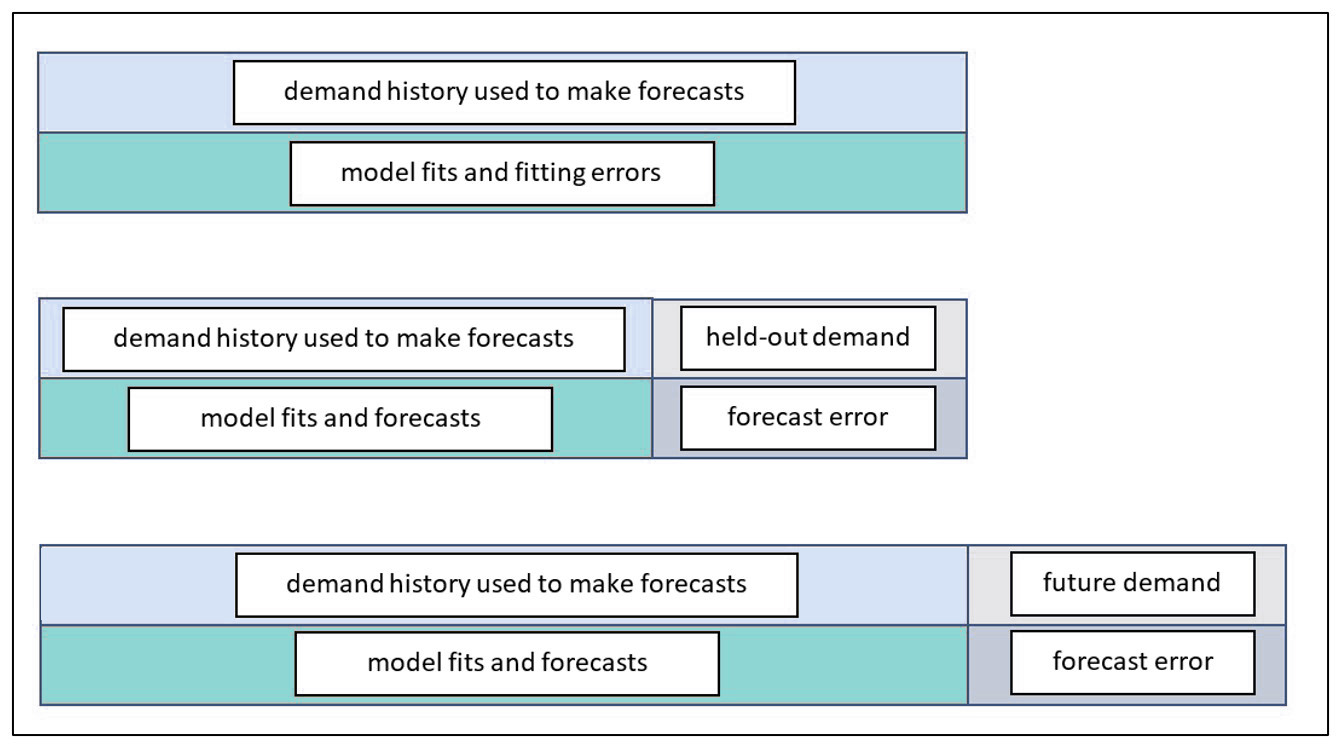
Figure 1: Three ways to assess forecast error

The top panel of Figure 1 depicts the way forecast error was assessed back in the early 1980’s before we moved the state of the art to the scheme shown in the middle panel. In the old days, forecasts were assessed on the same data used to compute the forecasts. After a model was fit to the data, the errors computed were not for model forecasts but for model fits. The difference is that forecasts are for future values, while fits are for concurrent values. For example, suppose the forecasting model is a simple moving average of the three most recent observations. At time 3, the model computes the average of observations 1, 2, and 3. This average would then be compared to the observed value at time 3. We call this cheating because the observed value at time 3 got a vote on what the forecast should be at time 3. A true forecast assessment would compare the average of the first three observations to the value of the next, fourth, observation. Otherwise, the forecaster is left with an overly optimistic assessment of forecast accuracy.

The bottom panel of Figure 1 shows the best way to assess forecast accuracy. In this schema, all the historical demand data are used to fit a model, which is then used to forecast future, unknown demand values. Eventually, the future unfolds, the true future values reveal themselves, and actual forecast errors can be computed. This is the gold standard. This information populates the “forecasts versus actuals” report in our software.

The middle panel depicts a useful halfway measure. The problem with the gold standard is that you must wait to learn how well your chosen forecasting methods perform. This delay does not help when you are required to choose, in the moment, which forecasting method to use for each item. Nor does it provide a timely estimate of the forecast uncertainty you will experience, which is important for risk management such as forecast hedging. The middle way is based on hold-out analysis, which excludes (“holds out”) the most recent observations and asks the forecasting method to do its work without knowing those ground truths. Then the forecasts based on the foreshortened demand history can be compared to the held-out actual values to get an honest assessment of forecast error.

You may remember the story of Goldilocks from your long-ago youth. Sometimes the porridge was too hot, sometimes it was too cold, but just once it was just right. Now that we are adults, we can translate that fairy tale into a professional principle for inventory planning: There can be too little or too much inventory, and there is some Goldilocks level that is “just right.” This blog is about finding that sweet spot.

To illustrate our supply chain fable, consider this example. Imagine that you sell service parts to keep your customers systems up and running. You offer a particular service part that costs you $100 to make but sells for a 20% markup. You can make $20 on each unit you sell, but you don’t get to keep the whole $20 because of the inventory operating costs you bear to be able to sell the part. There are holding costs to keep the part in good repair while in stock and ordering costs to replenish units you sell. Finally, sometimes you lose revenue from lost sales due to stockouts.  

These operating costs can be directly related to the way you manage the part in inventory. For our example, assume you use a (Q,R) inventory policy, where Q is the replenishment order quantity and R is the reorder point. Assume further that the reason you are not making $30 per unit is that you have competitors, and customers will get the part from them if they can’t get it from you.

Both your revenue and your costs depend in complex ways on your choices for Q and R. These will determine how much you order, when and therefore how often you order, how often you stock out and therefore how many sales you lose, and how much cash you tie up in inventory. It is impossible to cost out these relationships by guesswork, but modern software can make the relationships visible and calculate the dollar figures you need to guide your choice of values for Q and R. It does this by running detailed, fact-based, probabilistic simulations that predict costs and performance by averaging over a large number of realistic demand scenarios.  

With these results in hand, you can work out the margin associated with (Q,R) values using the simple formula

Margin = (Demand – Lost Sales) x Profit per unit sold – Ordering Costs – Holding Costs.

In this formula, Lost Sales, Ordering Costs and Holding Costs are dependent on reorder point R and order quantity Q.

Figure 1 shows the result of simulations that fixed Q at 25 units and varied R from 10 to 30 in steps of 5. While the curve is rather flat on top, you would make the most money by keeping on-hand inventory around 25 units (which corresponds to setting R = 20). More inventory, despite a higher service level and fewer lost sales, would make a little less money (and ties up a lot more cash), and less inventory would make a lot less.

Figure 1: Showing that there can be too little or too much inventory on hand

Without relying on the inventory simulation software, we would not be able to discover

• a) that it is possible to carry too little and too much inventory
• b) what the best level of inventory is
• c) how to get there by proper choices of reorder point R and order quantity Q.

Without an explicit understanding of the above, companies will make daily inventory decisions relying on gut feel and averaging based rule of thumb methods. The tradeoffs described here are not exposed and the resulting mix of inventory yields a far lower return forfeiting hundreds of thousands to millions per year in lost profits.  So be like Goldilocks.  With the right systems and software tools, you too can get it just right!