
BACKGROUND
Most of Smart Software’s blogs, webinars and white papers describe the use of our software in “normal operations.” This one is about “irregular operations.” Smart Software is in the process of adapting our products to help you cope with your own irregular ops. This is a preview.
I first heard the term “irregular operations” when serving a sabbatical tour at the U.S. Federal Aviation Administration in Washington, DC. The FAA abbreviates the term to “IROPS” and uses it to describe situations in which weather, mechanical problems or other issues disrupt the normal flow of aircraft.
Smart Inventory Optimization® (“SIO”) currently works to provide what are known as “steady state” policies for managing inventory items. That means, for instance, that SIO automatically calculates values for reorder points (ROP’s) and order quantities (OQ’s) that are meant to last for the foreseeable future. It computes these values based on simulations of daily operations that extend years into the future. If and when the unforeseeable happens, our regime change detection method reacts by removing obsolete data and allowing recalculation of the ROP’s and OQ’s.
We often note the increasing speed of business, which shortens the duration of the “foreseeable future.” Some of our customers are now adopting shorter planning horizons, such as moving from quarterly to monthly plans. One side effect of this change is that IROPS have become more consequential. If a plan is based on three simulated years of daily demand, one odd event, like a large surprise order, doesn’t matter much in the grand scheme of things. But if the planning horizon is very short, one big surprise demand can have a major effect on key performance indicators (KPI’s) computed over a shorter interval – there is no time for “averaging out”. The planner may be forced to place an emergency replenishment order to deal with the disruption. When should the order be placed to do the most good? How big should it be?
SCENARIO: NORMAL OPS
To make this concrete, consider the following scenario. Tom’s Spares, Inc. provides critical service parts to its customers, including SKU723, a replacement circuit board sold under the trade name WIDGET. Demand for WIDGET is intermittent, with less than one unit demanded per day. Tom’s Spares orders WIDGETs from Acme Products, who take either 7 or 10 days to fulfill replenishment orders.
Tom’s Spares operates with a short inventory planning horizon of 28 days. The company operates in a competitive environment with impatient customers who only grudgingly accept backorders. Tom’s policy is to set ROP’s and OQ’s to keep inventory lean while maintaining a fill rate of at least 90%. Management monitors KPI’s on a monthly basis. In the case of WIDGETS, these KPI targets are currently met using an ROP=3 and an OQ=4, resulting in an average on hand of about 4 units and average fill rate of 96%. Tom’s Spares has a pretty good thing going for WIDGETS.
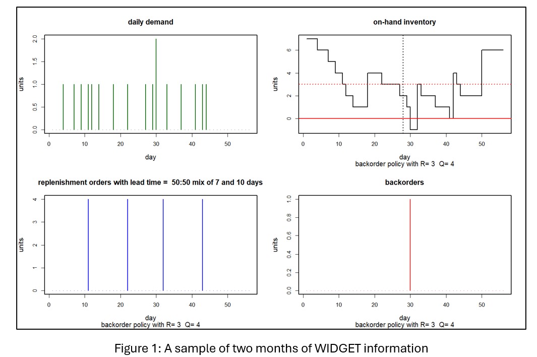
Figure 1 shows two months of WIDGET information. The top left panel shows daily unit demand. The top right shows daily units on hand. The bottom left panel shows the timing and size of replenishment orders back to Acme Products. The bottom right shows units backordered due to stockouts. In this simulation, daily demand was either 0 or 1, with one demand of 2 units. On hand units began the month at 7 and never dropped below 1, though in the next month there was a stockout resulting in a single unit on backorder. Over the two months, there were 4 replenishment orders of 4 units each sent to Acme, all of which arrived during the two-month simulation period.
GOOD TROUBLE DISRUPTS NORMAL OPS
Now we add some “good trouble” to the scenario: An unusually large order arises part way through the planning period. It’s “good” because more demand implies more revenue. But it’s “trouble” because the normal ops inventory control parameters (ROP=3, OQ=4) were not chosen to cope with this situation. The spike in demand might be so big, and so disadvantageously timed, as to overwhelm the inventory system, creating stockouts and their attendant backorders. The KPI report to management for such a month would not be pretty.
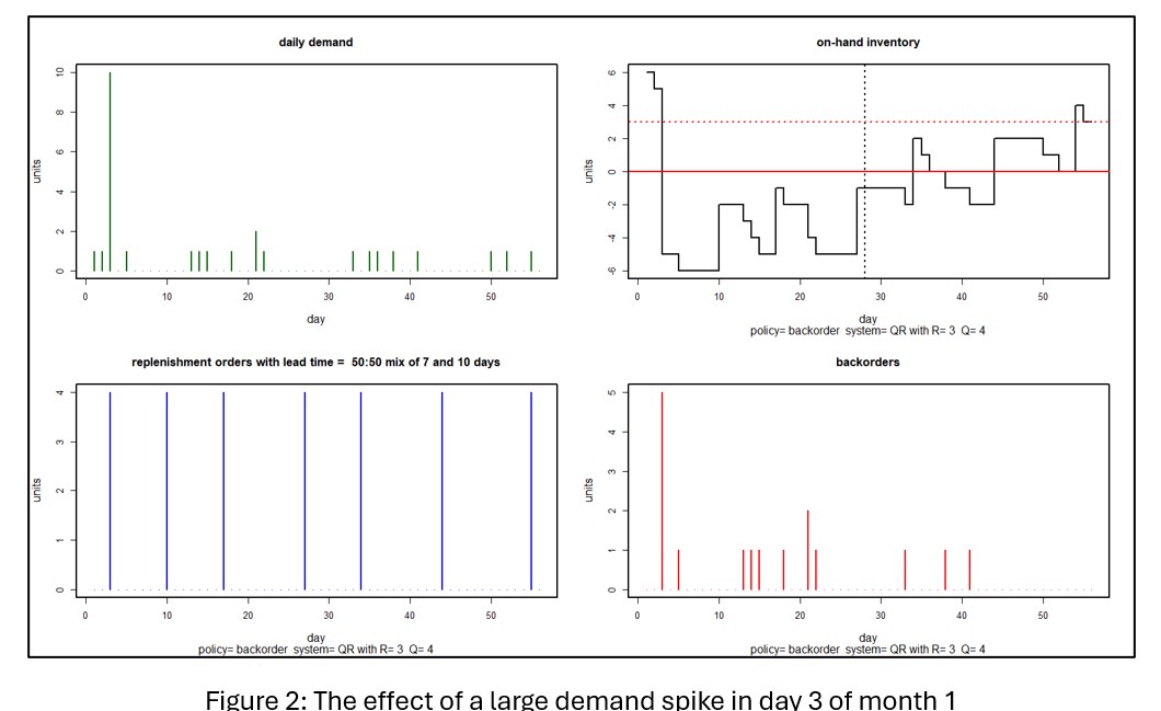
Figure 2 shows a scenario in which a demand spike of 10 units hits in the third day of the planning period. In this case, the spike puts the inventory under water for the rest of the month and creates a cascade of backorders extending into the next month. Averaging over 1,000 simulations, month 1 KPI’s show an average on hand of 0.6 units and a miserable 44% fill rate.
FIGHTING BACK WITH IRREGULAR OPERATIONS
Tom’s Spares can respond to an irregular situation with an irregular move by creating an emergency replenishment order. To do it right, they have to think about (a) when to place the order (b) how big the order should be and (c) whether to expedite the order.
The timing question seems obvious: react as soon as the order hits. However, if the customer were to provide early warning, Tom’s Spares could order early and be in better position to limit the disruption from the spike. However, if communication between Tom’s and the customer making the big order is spotty, then the customer might give Tom’s a heads-up later or not at all.
The size of the special order seems obvious too: pre-order the required number of units. But that works best if Tom’s Spares knows when the demand spike will hit. If not, it might be a good idea to order extra to limit the duration of any backorders. In general, the less early warning provided, the larger the order Tom’s should make. This relationship could be explored with simulation, of course.
The arrival of the replenishment order could be left to the usual operation of Acme Products. In the simulations above, Acme was equally likely to respond in 7 or 14 days. For a 28-day planning horizon, taking a risk on getting a 14-day response might be asking for trouble, so it may be especially worthwhile for Tom’s to pay Acme for expedited shipping. Maybe overnight, but possibly something cheaper but still relatively fast.
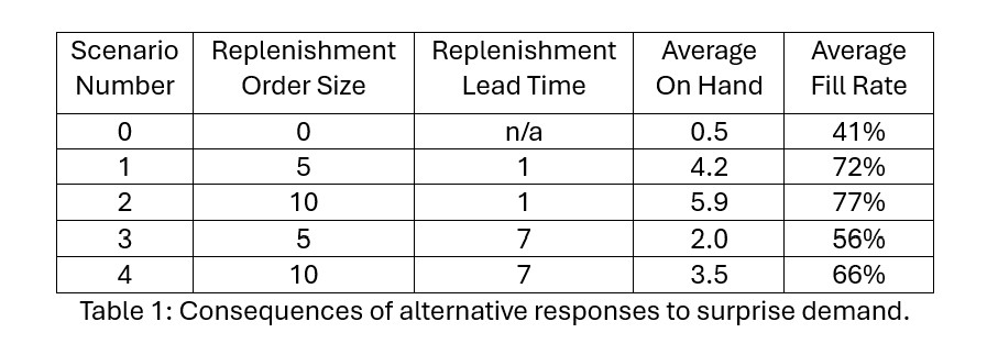
We explored a few more scenarios using simulation. Table 1 shows the results. Scenarios 1-4 assume a surprise additional demand of 10 units arrives on Day 3, triggering an immediate order for additional replenishment. The size and lead time of the replenishment order varies.
Scenario 0 shows that doing nothing in response to the surprise demand leads to an abysmal 41% fill rate for that month; not shown is that this result sets of the next month for continued poor performance. Regular operations won’t do well. The planner must do something to respond to the anomalous demand.
Doing something in response involves making a one-time emergency replenishment order. The planner must choose the size and timing of that order. Scenarios 1 and 3 depict “half sized” replenishments. Scenarios 1 and 2 depict overnight replenishments, while scenarios 3 and 4 depict guaranteed one week response.
The results make clear that immediate response is more important than the size of the replenishment order for restoring the Fill Rate. Overnight replenishment produces fill rates in the 70% range, while one-week replenishment lead time drops the fill rate into the mid-50% to mid-60% range.
TAKEAWAYS
Inventory management software is expanding from its traditional focus on normal ops to an additional focus on irregular ops (IROPS). This evolution has been made possible by the development of new statistical methods for generating demand scenarios at a daily level.
We considered one IROPS situation: surprise arrival of an anomalously large demand. Daily simulations provided guidance about the timing and size of an emergency replenishment order. Results from such an analysis provide inventory planners with critical backup by estimating the results of alternative interventions that their experience suggests to them.