Supply Chain Math: Don’t Bring a Knife to a Gunfight

Whether you understand it in detail yourself or rely on trustworthy software, math is a fact of life for anyone in inventory management and demand forecasting who is hoping to remain competitive in the modern world.

At a conference recently, the lead presenter in an inventory management workshop proudly proclaimed that he had no need for “high-fallutin’ math”, which was explained to mean anything beyond sixth-grade math.

Math is not everyone’s first love. But if you really care about doing your job well, you can’t approach the work with a grade school mentality. Supply chain tasks like demand forecasting and inventory management are inherently mathematical. The blog associated with edX, a premier site for online college course material, has a great post on this topic, at https://www.mooc.org/blog/how-is-math-used-in-supply-chain. Let me quote the first bit:

Math and the supply chain go hand and hand. As supply chains grow, increasing complexity will drive companies to look for ways to manage large-scale decision-making. They can’t go back to how supply chains were 100 years ago—or even two years ago before the pandemic. Instead, new technologies will help streamline and manage the many moving parts. The logistics skills, optimization technologies, and organizational skills used in supply chain all require mathematics.

Our customers don’t need to be experts in supply chain math, they just need to be able to wield the software that contains the math. Software combines users’ experience and subject matter expertise to produce results that make the difference between success and failure. To do its job, the software can’t stop at sixth-grade math; it needs probability, statistics, and optimization theory.

It’s up to us software vendors to package the math in such a way that what goes into the calculations is all that is relevant, even if complicated; and that what comes out is clear, decision-relevant, and defensible when you must justify your recommendations to higher management.

Sixth-grade math can’t warn you when the way you propose to manage a critical spare part will mean a 70% chance of falling short of your item availability target. It can’t tell you how best to adjust your reorder points when a supplier calls and says, “We have a delivery problem.” It can’t save your skin when there is a surprisingly large order and you have to quickly figure out the best way to set up some expedited special orders without busting the operating budget.

So, respect the folk wisdom and don’t bring a knife to a gunfight.


The Supply Chain Blame Game: Top 3 Excuses for Inventory Shortage and Excess

1. Blaming Shortages on Lead Time Variability
Suppliers will often be late, sometimes by a lot. Lead time delays and supply variability are supply chain facts of life, yet inventory carrying organizations are often caught by surprise when a supplier is late.  An effective inventory planning process embraces these facts of life and develops policies that effectively account for this uncertainty.  Sure, there will be times when lead time delays come out of nowhere.  But most often the stocking policies like reorder points, safety stocks, and Min/Max levels aren’t recalibrated often enough to catch changes in the lead time over time.  Many companies only review the reorder point after it has been breached, instead of recalibrating after each new lead time receipt.  We’ve observed situations where the Min/Max settings are only recalibrated annually or are even entirely manual.  If you have a mountain of parts using old Min/Max levels and associated lead times that were relevant a year ago, it should be no surprise that you don’t have enough inventory to hold you until the next order arrives.


2. Blaming Excess on Bad Sales/Customer Forecasts
Forecasts from your customers or your sales team are often intentionally over-estimated to ensure supply, in response to past inventory shortages where they were left out to dry. Or, the demand forecasts are inaccurate simply because the sales team doesn’t really know what their customer demand is going to be but are forced to give a number. Demand Variability is another supply chain fact of life, so planning processes need to do a better job account for it.  Why should rely on sales teams to forecast when they best serve the company by selling? Why bother playing the game of feigning acceptance of customer forecasts when both sides know it is often nothing more than a WAG?  A better way is to accept the uncertainty and agree on a degree of stockout risk that is acceptable across groups of items.  Once the stockout risk is agreed to, you can generate an accurate estimate of the safety stock needed to counter the demand variability.  The catch is getting buy-in, since you may not be able to afford super high service levels across all items.  Customers must be willing to pay a higher price per unit for you to deliver extremely high service levels.  Sales people must accept that certain items are more likely to have backorders if they prioritize inventory investment on other items.  Using a consensus safety stock process ensures you are properly buffering and setting the right expectations.  When you do this, you free all parties from having to play the prediction game they were not equipped to play in the first place.


3. Blaming Problems on Bad Data
“Garbage In/Garbage Out” is a common excuse for why now is not the right time to invest in planning software. Of course, it is true that if you feed bad data into a model, you won’t get good results, but here’s the thing:  someone, somewhere in the organization is planning inventory, building a forecast, and making decisions on what to purchase. Are they doing this blindly, or are they using data they have curated in a spreadsheet to help them make inventory planning decisions? Hopefully, the latter.  Combine that internal knowledge with software, automating data import from the ERP, and data cleansing.  Once harmonized, your planning software will provide continually updated, well-structured demand and lead time signals that now make effective demand forecasting and inventory optimization possible.  Smart Software cofounder Tom Willemain wrote in an IBF newsletter that “many data problems derive from data having been neglected until a forecasting project made them important.” So, start that forecasting project, because step one is making sure that “what goes in” is a pristine, documented, and accurate demand signal.


Call an Audible to Proactively Counter Supply Chain Noise


You know the situation: You work out the best way to manage each inventory item by computing the proper reorder points and replenishment targets, then average demand increases or decreases, or demand volatility changes, or suppliers’ lead times change, or your own costs change. Now your old policies (reorder points, safety stocks, Min/Max levels, etc.)  have been obsoleted – just when you think you’d got them right.   Leveraging advanced planning and inventory optimization software gives you the ability to proactively address ever-changing outside influences on your inventory and demand.  To do so, you’ll need to regularly recalibrate stocking parameters based on ever-changing demand and lead times.

Recently, some potential customers have expressed concern that by regularly modifying inventory control parameters they are introducing “noise” and adding complication to their operations. A visitor to our booth at last week’s Microsoft Dynamics User Group Conference commented:

“We don’t want to jerk around the operations by changing the policies too often and introducing noise into the system. That noise makes the system nervous and causes confusion among the buying team.”

This view is grounded in yesterday’s paradigms.  While you should generally not change an immediate production run, ignoring near-term changes to the policies that drive future production planning and order replenishment will wreak havoc on your operations.   Like it or not, the noise is already there in the form of extreme demand and supply chain variability.  Fixing replenishment parameters, updating them infrequently, or only reviewing at the time of order means that your Supply Chain Operations will only be able to react to problems rather than proactively identify them and take corrective action.

Modifying the policies with near-term recalibrations is adapting to a fluid situation rather than being captive to it.  We can look to this past weekend’s NFL games for a simple analogy. Imagine the quarterback of your favorite team consistently refusing to call an audible (change the play just before the ball is snapped) after seeing the defensive formation.  This would result in lots of missed opportunities, inefficiency, and stalled drives that could cost the team a victory.  What would you want your quarterback to do?

Demand, lead times, costs, and business priorities often change, and as these last 18 months have proved they often change considerably.  As a Supply Chain leader, you have a choice:  keep parameters fixed resulting in lots of knee-jerk expedites and order cancellations, or proactively modify inventory control parameters.  Calling the audible by recalibrating your policies as demand and supply signals change is the right move.

Here is an example. Suppose you are managing a critical item by controlling its reorder point (ROP) at 25 units and its order quantity (OQ) at 48. You may feel like a rock of stability by holding on to those two numbers, but by doing so you may be letting other numbers fluctuate dramatically.  Specifically, your future service levels, fill rates, and operating costs could all be resetting out of sight while you fixate on holding onto yesterday’s ROP and OQ.  When the policy was originally determined, demand was stable and lead times were predictable, yielding service levels of 99% on an important item.   But now demand is increasing and lead times are longer.  Are you really going to expect the same outcome (99% service level) using the same sets of inputs now that demand and lead times are so different?  Of course not.  Suppose you knew that given the recent changes in demand and lead time, in order to achieve the same service level target of 99%, you had to increase the ROP to 35 units.  If you were to keep the ROP at 25 units your service level would fall to 92%.  Is it better to know this in advance or to be forced to react when you are facing stockouts?

What inventory optimization and planning software does is make visible the connections between performance metrics like service rate and control parameters like ROP and ROQ. The invisible becomes visible, allowing you to make reasoned adjustments that keep your metrics where you need them to be by adjusting the control levers available for your use.  Using probabilistic forecasting methods will enable you to generate Key Performance Predictions (KPPs) of performance and costs while identifying near-term corrective actions such as targeted stock movements that help avoid problems and take advantage of opportunities. Not doing so puts your supply chain planning in a straightjacket, much like the quarterback who refuses to audible.

Admittedly, a constantly-changing business environment requires constant vigilance and occasional reaction. But the right inventory optimization and demand forecasting software can recompute your control parameters at scale with a few mouse clicks and clue your ERP system how to keep everything on course despite the constant turbulence.  The noise is already in your system in the form of demand and supply variability.  Will you proactively audible or stick to an older plan and cross your fingers that things will work out fine?


Leave a Comment
Related Posts
Why Inventory Planning Shouldn’t Rely Exclusively on Simple Rules of Thumb

Why Inventory Planning Shouldn’t Rely Exclusively on Simple Rules of Thumb

For too many companies, a critical piece of data fact-finding ― the measurement of demand uncertainty ― is handled by simple but inaccurate rules of thumb. For example, demand planners will often compute safety stock by a user-defined multiple of the forecast or historical average. Or they may configure their ERP to order more when on hand inventory gets to 2 x the average demand over the lead time for important items and 1.5 x for less important ones. This is a huge mistake with costly consequences.

Why MRO Businesses Should Care About Excess Inventory

Why MRO Businesses Should Care About Excess Inventory

Do MRO companies genuinely prioritize reducing excess spare parts inventory? From an organizational standpoint, our experience suggests not necessarily. Boardroom discussions typically revolve around expanding fleets, acquiring new customers, meeting service level agreements (SLAs), modernizing infrastructure, and maximizing uptime. In industries where assets supported by spare parts cost hundreds of millions or generate significant revenue (e.g., mining or oil & gas), the value of the inventory just doesn’t raise any eyebrows, and organizations tend to overlook massive amounts of excessive inventory.

Constructive Play with Digital Twins

Constructive Play with Digital Twins

Those of you who track hot topics will be familiar with the term “digital twin.” Those who have been too busy with work may want to read on and catch up. While there are several definitions of digital twin, here’s one that works well: A digital twin is a dynamic virtual copy of a physical asset, process, system, or environment that looks like and behaves identically to its real-world counterpart. A digital twin ingests data and replicates processes so you can predict possible performance outcomes and issues that the real-world product might undergo.

An Example of Simulation-Based Multiechelon Inventory Optimization

Managing the inventory in a single facility is difficult enough, but the problem becomes much more complex when there are multiple facilities arrayed in multiple echelons. The complexity arises from the interactions among the echelons, with demands at the lower levels bubbling up and any shortages at the higher levels cascading down.

If each of the facilities were to be managed in isolation, standard methods could be used, without regard to interactions, to set inventory control parameters such as reorder points and order quantities. However, ignoring the interactions between levels can lead to catastrophic failures. Experience and trial and error allow the design of stable systems, but that stability can be shattered by changes in demand patterns or lead times or by the addition of new facilities. Coping with such changes is greatly aided by advanced supply chain analytics, which provide a safe “sandbox” within which to test out proposed system changes before deploying them. This blog illustrates that point.


The Scenario

To have some hope of discussing this problem usefully, this blog will simplify the problem by considering the two-level hierarchy pictured in Figure 1. Imagine the facilities at the lower level to be warehouses (WHs) from which customer demands are meant to be satisfied, and that the inventory items at each WH are service parts sold to a wide range of external customers.


Fact and Fantasy in Multiechelon Inventory Optimization

Figure 1: General structure of one type of two-level inventory system

Imagine the higher level to consist of a single distribution center (DC) which does not service customers directly but does replenish the WHs. For simplicity, assume the DC itself is replenished from a Source that always has (or makes) sufficient stock to immediately ship parts to the DC, though with some delay. (Alternatively, we could consider the system to have retail stores supplied by one warehouse).

Each level can be described in terms of demand levels (treated as random), lead times (random), inventory control parameters (here, Min and Max values) and shortage policy (here, backorders allowed).


The Method of Analysis

The academic literature has made progress on this problem, though usually at the cost of simplifications necessary to facilitate a purely mathematical solution. Our approach here is more accessible and flexible: Monte Carlo simulation. That is, we build a computer program that incorporates the logic of the system operation. The program “creates” random demand at the WH level, processes the demand according to the logic of a chosen inventory policy, and creates demand for the DC by pooling the random requests for replenishment made by the WHs. This approach lets us observe many simulated days of system operation while watching for significant events like stockouts at either level.


An Example

To illustrate an analysis, we simulated a system consisting of four WHs and one DC. Average demand varied across the WHs. Replenishment from the DC to any WH took from 4 to 7 days, averaging 5.15 days. Replenishment of the DC from the Source took either 7, 14, 21 or 28 days, but 90% of the time it was either 21 or 28 days, making the average 21 days. Each facility had Min and Max values set by analyst judgement after some rough calculations.

Figure 2 shows the results of one year of simulated daily operation of this system. The first row in the figure shows the daily demand for the item at each WH, which was assumed to be “purely random”, meaning it had a Poisson distribution. The second row shows the on-hand inventory at the end of each day, with Min and Max values indicated by blue lines. The third row describes operations at the DC.  Contrary to the assumption of much theory, the demand into the DC was not close to being Poisson, nor was the demand out of the DC to the Source. In this scenario, Min and Max values were sufficient to keep item availability was high at each WH and at the DC, with no stockouts observed at any of the five facilities.


Click here to enlarge the image

Figure 2 - Simulated year of operation of a system with four WHs and one DC.

Figure 2 – Simulated year of operation of a system with four WHs and one DC.


Now let’s vary the scenario. When stockouts are extremely rare, as in Figure 2, there is often excess inventory in the system. Suppose somebody suggests that the inventory level at the DC looks a bit fat and thinks it would be good idea to save money there. Their suggestion for reducing the stock at the DC is to reduce the value of the Min at the DC from 100 to 50. What happens? You could guess, or you could simulate.

Figure 3 shows the simulation – the result is not pretty. The system runs fine for much of the year, then the DC runs out of stock and cannot catch up despite sending successively larger replenishment orders to the Source. Three of the four WHs descend into death spirals by the end of the year (and WH1 follows thereafter). The simulation has highlighted a sensitivity that cannot be ignored and has flagged a bad decision.


Click here to enlarge image

Figure 3 - Simulated effects of reducing the Min at the DC.

Figure 3 – Simulated effects of reducing the Min at the DC.


Now the inventory managers can go back to the drawing board and test out other possible ways to reduce the investment in inventory at the DC level. One move that always helps, if you and your supplier can jointly make it happen, is to create a more agile system by reducing replenishment lead time. Working with the Source to insure that the DC always gets its replenishments in either 7 or 14 days stabilizes the system, as shown in Figure 4.


Click here to enlarge image

Figure 4 - Simulated effects of reducing the lead time for replenishing the DC.

Figure 4 – Simulated effects of reducing the lead time for replenishing the DC.


Unfortunately, the intent of reducing the inventory at the DC has not been achieved. The original daily inventory count was about 80 units and remains about 80 units after reducing the DC’s Min and drastically improving the Source-to-DC lead time. But with the simulation model, the planning team can try out other ideas until they arrive at a satisfactory redesign. Or, given that Figure 4 shows the DC inventory starting to flirt with zero, they might think it prudent to accept the need for an average of about 80 units at the DC and look for ways to trim inventory investment at the WHs instead.


The Takeaways

  1. Multiechelon inventory optimization (MEIO) is complex. Many factors interact to produce system behaviors that can be surprising in even simple two-level systems.
  2. Monte Carlo simulation is a useful tool for planners who need to design new systems or tweak existing systems.


Leave a Comment
Related Posts
Why Inventory Planning Shouldn’t Rely Exclusively on Simple Rules of Thumb

Why Inventory Planning Shouldn’t Rely Exclusively on Simple Rules of Thumb

For too many companies, a critical piece of data fact-finding ― the measurement of demand uncertainty ― is handled by simple but inaccurate rules of thumb. For example, demand planners will often compute safety stock by a user-defined multiple of the forecast or historical average. Or they may configure their ERP to order more when on hand inventory gets to 2 x the average demand over the lead time for important items and 1.5 x for less important ones. This is a huge mistake with costly consequences.

Why MRO Businesses Should Care About Excess Inventory

Why MRO Businesses Should Care About Excess Inventory

Do MRO companies genuinely prioritize reducing excess spare parts inventory? From an organizational standpoint, our experience suggests not necessarily. Boardroom discussions typically revolve around expanding fleets, acquiring new customers, meeting service level agreements (SLAs), modernizing infrastructure, and maximizing uptime. In industries where assets supported by spare parts cost hundreds of millions or generate significant revenue (e.g., mining or oil & gas), the value of the inventory just doesn’t raise any eyebrows, and organizations tend to overlook massive amounts of excessive inventory.

Constructive Play with Digital Twins

Constructive Play with Digital Twins

Those of you who track hot topics will be familiar with the term “digital twin.” Those who have been too busy with work may want to read on and catch up. While there are several definitions of digital twin, here’s one that works well: A digital twin is a dynamic virtual copy of a physical asset, process, system, or environment that looks like and behaves identically to its real-world counterpart. A digital twin ingests data and replicates processes so you can predict possible performance outcomes and issues that the real-world product might undergo.

Fact and Fantasy in Multiechelon Inventory Optimization

For most small-to-medium manufacturers and distributors, single-level or single-echelon inventory optimization is at the cutting edge of logistics practice. Multi-echelon inventory optimization (“MEIO”) involves playing the game at an even higher level and is therefore much less common. This blog is the first of two. It aims to explain what MEIO is, why standard MEIO theories break down, and how probabilistic modeling through scenario simulation can restore reality to the MEIO process. The second blog will show a particular example.


Definition of Inventory Optimization

An inventory system is built on a set of design choices.

The first choice is the policy for responding to stockouts: Do you just lose the sale to a competitor, or can you convince the customer to accept a backorder? The former is more common with distributors than manufacturers, but this may not be much of a choice since customers may dictate the answer.

The second choice is the inventory policy. These divide into “continuous review” and “periodic review” policies, with several options within each type. You can link to a video tutorial describing several common inventory policies here.  Perhaps the most efficient is known to practitioners as “Min/Max” and to academics as (s, S) or “little S, Big S.” We use this policy in the scenario simulations below. It works as follows: When on-hand inventory drops to or below the Min (s), an order is placed for replenishment. The size of the order is the gap between the on-hand inventory and the Max (S), so if Min is 10, Max is 25 and on-hand is 8, it’s time for an order of 25-8 = 17 units.

The third choice is to decide on the best values of the inventory policy “parameters”, e.g., the values to use for Min and Max. Before assigning numbers to Min and Max, you need clarity on what “best” means for you. Commonly, best means choices that minimize inventory operating costs subject to a floor on item availability, expressed either as Service Level or Fill Rate. In mathematical terms, this is a “two-dimensional constrained integer optimization problem”. “Two-dimensional” because you have to pick two numbers: Min and Max. “Integer” because Min and Max have to be whole numbers. “Constrained” because you must pick Min and Max values that give a high-enough level of item availability such as service levels and fill rates. “Optimization” because you  want to get there with the lowest operating cost (operating cost combines holding, ordering and shortage costs).


Multiechelon Inventory Systems

The optimization problem becomes more difficult in multi-echelon systems. In a single-echelon system, each inventory item can be analyzed in isolation: one pair of Min/Max values per SKU. Because there are more parts to a multiechelon system, there is a bigger computational problem.

Figure 1 shows a simple two-level system for managing a single SKU. At the lower level, demands arrive at multiple warehouses. When those are in danger of stocking out, they are resupplied from a distribution center (DC). When the DC itself is in danger of stocking out, it is supplied by some outside source, such as the manufacturer of the item.

The design problem here is multidimensional: We need Min and Max values for 4 warehouses and for the DC, so the optimization occurs in 4×2+1×2=10 dimensions. The analysis must take account of a multitude of contextual factors:

  • The average level and volatility of demand coming into each warehouse.
  • The average and variability of replenishment lead times from the DC.
  • The average and variability of replenishment lead times from the source.
  • The required minimum service level at the warehouses.
  • The required minimum service level at the DC.
  • The holding, ordering and shortage costs at each warehouse.
  • The holding, ordering and shortage costs at the DC.

As you might expect, seat-of-the-pants guesses won’t do well in this situation. Neither will trying to simplify the problem by analyzing each echelon separately. For instance, stockouts at the DC increase the risk of stockouts at the warehouse level and vice versa.

This problem is obviously too complicated to try to solve without help from some sort of computer model.


Why Standard Inventory Theory is Bad Math

With a little looking, you can find models, journal articles and book about MEIO. These are valuable sources of information and insight, even numbers. But most of them rely on the expedient of over-simplifying the problem to make it possible to write and solve equations. This is the “Fantasy” referred to in the title.

Doing so is a classic modeling maneuver and is not necessarily a bad idea. When I was a graduate student at MIT, I was taught the value of having two models: a small, rough model to serve as a kind of sighting scope and a larger, more accurate model to produce reliable numbers. The smaller model is equation-based and theory-based; the bigger model is procedure-based and data-based, i.e., a detailed system simulation. Models based on simple theories and equations can produce bad numerical estimates and even miss whole phenomena. In contrast, models based on procedures (e.g., “order up to the Max when you breach the Min”) and facts (e.g., the last 3 years of daily item demand) will require a lot more computing but give more realistic answers. Luckily, thanks to the cloud, we have a lot of computing power at our fingertips.

Perhaps the greatest modeling “sin” in the MEIO literature is the assumption that demands at all echelons can be modeled as purely random Poisson processes. Even if it were true at the warehouse level, it would be far from true at the DC level. The Poisson process is the “white rat of demand modeling” because it is simple and permits more paper-and-pencil equation manipulation. Since not all demands are Poisson shaped, this results in unrealistic recommendations.


Scenario-based Simulation Optimization

To get realism, we must get down into the details of how the inventory systems operate at each echelon. With few limits except those imposed by hardware such as size of memory, computer programs can keep up any level of complexity. For instance, there is no need to assume that each of the warehouses faces identical demand streams or has the same costs as all the others.

A computer simulation works as follows.

  1. The real-world demand history and lead time history are gathered for each SKU at each location.
  2. Values of inventory parameters (e.g., Min and Max) are selected for trial.
  3. The demand and replenishment histories are used to create scenarios depicting inputs to the computer program that encodes the rules of operation of the system.
  4. The inputs are used to drive the operation of a computer model of the system with the chosen parameter values over a long period, say one year.
  5. Key performance indicators (KPI’s) are calculated for the simulated year.
  6. Steps 2-5 are repeated many times and the results averaged to link parameter choices to system performance.
  7.  

Inventory optimization adds another “outer loop” to the calculations by systematically searching over the possible values of Min and Max. Among those parameter pairs that satisfy the item availability constraint, further search identifies the Min and Max values that result in the lowest operating cost.

Fact and Fantasy in Multiechelon Inventory Optimization

Figure 1: General structure of one type of two-level inventory system


Stay Tuned for our next Blog

COMING SOON. To see an example of a simulation of the system in Figure 1, read the second blog on this topic


Leave a Comment
Related Posts
Why Inventory Planning Shouldn’t Rely Exclusively on Simple Rules of Thumb

Why Inventory Planning Shouldn’t Rely Exclusively on Simple Rules of Thumb

For too many companies, a critical piece of data fact-finding ― the measurement of demand uncertainty ― is handled by simple but inaccurate rules of thumb. For example, demand planners will often compute safety stock by a user-defined multiple of the forecast or historical average. Or they may configure their ERP to order more when on hand inventory gets to 2 x the average demand over the lead time for important items and 1.5 x for less important ones. This is a huge mistake with costly consequences.

Why MRO Businesses Should Care About Excess Inventory

Why MRO Businesses Should Care About Excess Inventory

Do MRO companies genuinely prioritize reducing excess spare parts inventory? From an organizational standpoint, our experience suggests not necessarily. Boardroom discussions typically revolve around expanding fleets, acquiring new customers, meeting service level agreements (SLAs), modernizing infrastructure, and maximizing uptime. In industries where assets supported by spare parts cost hundreds of millions or generate significant revenue (e.g., mining or oil & gas), the value of the inventory just doesn’t raise any eyebrows, and organizations tend to overlook massive amounts of excessive inventory.

Constructive Play with Digital Twins

Constructive Play with Digital Twins

Those of you who track hot topics will be familiar with the term “digital twin.” Those who have been too busy with work may want to read on and catch up. While there are several definitions of digital twin, here’s one that works well: A digital twin is a dynamic virtual copy of a physical asset, process, system, or environment that looks like and behaves identically to its real-world counterpart. A digital twin ingests data and replicates processes so you can predict possible performance outcomes and issues that the real-world product might undergo.

Assessing How Suppliers Influence Your Inventory Costs

The Smart Forecaster

 Pursuing best practices in demand planning,

forecasting and inventory optimization

Software for inventory optimization is most often used to crank out the analytical results you need to run your day-to-day business, such as Reorder Points (also known as Mins) and Order Quantities. This specialized software helps you find the sweet spot that balances inventory costs against item availability during routine operations.

Inventory optimization software can also be used to perform “what-if” analyses on scenarios that describe changes from your current operating environment. What-if analysis (also called “sensitivity analysis”) lets you elevate your thinking from the tactical to the strategic. It helps you imagine how you should change your operations to adapt to potential changes in your operating environment. These changes might be negative pressures imposed on you from the outside, or they might result from your own positive actions. In this blog, we provide an example of how to conduct “what-analysis” on lead times and order quantities.  Outputs from the analysis can be used by the business to assess the impact of these changes on inventory costs and service level performance.

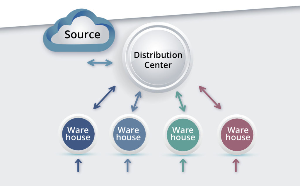
How Suppliers Limit Your Freedom of Maneuver


Discussing with our customers the data inputs required by inventory optimization software, we noted that suppliers are a prominent influence on their operations. We leave aside for now such important topics as sharing demand forecasts with suppliers and working out responses to supply chain disruptions, such as Hurricane Matthew last year in the southeastern US. Instead, we focus on two more common ways that suppliers influence producers’ inventory costs: replenishment lead times and restrictions on order quantities.

Replenishment lead time is the number of days that elapse between inventory reaching or breaching a reorder point and the appearance of replenishment units in stock. Some portion of lead time is internal to the producer, perhaps due to slow reactions in a purchasing department. The rest of lead time is down to the supplier. In this discussion, we assume that suppliers’ contribution to lead times might be changed, for better or for worse. (But the same results could apply to changes in producers’ contributions to lead times.)

The restrictions on order quantities that we consider are order minima and order multiples. You might want to order 3 units of some item, but the supplier might impose a minimum order size of 6 units, so your 3 unit order would have to become a 6 unit order. Or you might want to order 21 units, handily exceeding the minimum order size of 6 units, but if the supplier also has an order multiple of 6, meaning every order must be a multiple of 6 units, then your 21 unit order would have to be increased to 24 units.

Scenario Analyses


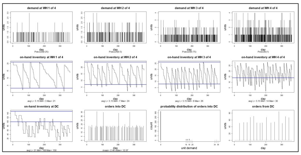
To illustrate the use of inventory optimization software for what-if analysis, we examine two sets of scenarios. In the first set, lead times are varied from -20% to +20% of their values in a baseline scenario. In the second set, results are computed first with no supplier restrictions, then with order minima only, and finally with a combination of order minima and order multiples. We use Smart Inventory Optimization software for the calculations.

The baseline scenario uses real-world data on 2,852 spare parts managed by a progressive public transit agency. These parts have an extremely heterogeneous mix of attributes. Their per unit costs range from $1 to $23,105, and their lead times vary between 1 day and 300 days. Over 24 months, the mean demand ranged from less than 1 unit per month to 1,508 units per month, with coefficients of variation ranging from a manageable 10% to a scary 2,171%. Furthermore, the supplier picture is also very complex, involving 293 unique vendors, supplying an average of about 10 parts each. This heterogeneity implies that a real-world optimization would pick and choose among items and vendors. However, for simplicity of exposition and to develop basic insights, our what-if scenarios in this example treat every item and vendor equally. Similarly, we assumed in the baseline that holding costs equaled 20% of the dollar value of an item and that every replenishment order had a fixed cost of $40.

We conducted two what-if experiments. The first examined the effects of changing lead times. The second examined the effects of introducing restrictions on order quantities. In each experiment, we recorded the effects of the changes on two operational metrics: average number of units in stock and average number of orders per year. In turn, these influenced four financial metrics: average dollar value of inventory, average holding cost, average ordering cost, and the sum of the last two, which is total inventory operating cost.

In all scenarios, reorder points were calculated so as to achieve 95% probability of avoiding stockouts while waiting for replenishment. Order quantities, in the absence of supplier restrictions, were computed as what we call “feasible EOQ”. EOQ is the classic “economic order quantity” taught in Inventory 101; it is computed from average demand, holding cost and ordering cost. Feasible EOQ adds an additional consideration: inventory dynamics. If the reorder point is very low, it is possible for EOQ to be too small to sustain a stable, positive level of inventory. In these cases, feasible EOQ increases the order quantity above the EOQ to insure that average inventory does not go negative.

Effects of Changing Lead Times

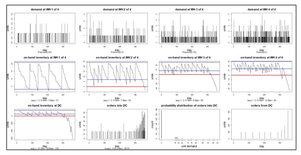
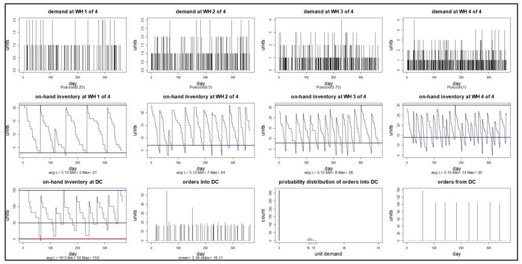
Table 1 shows the results of changing the lead times. Working around the base case, we changed every item’s lead time by -20%, -10%, +10% and +20%.

It is no surprise that reducing lead times reduced the required level of inventory and increasing them did the opposite. Both the average number of units and the associated dollar value behaved as expected. What may be surprising is that the effects were somewhat muted, i.e., an X percent change in lead time produced a less-than-X percent response. For instance, a 20% reduction in lead time produced only a 7.9% reduction in on-hand inventory and only a 12.0% reduction in the dollar value of those units. Furthermore, the effects of reductions and increases are asymmetric: a 20% increase in lead time led to just a 7.3% increase in units (vs 7.9%) and only a 9.6% increase in inventory value (vs 12.0%).

Similar attenuated and asymmetric results held for operating costs. A 20% reduction in lead time decreased total operating costs by 7.0%, but a 20% increase in lead time caused only a 5.1% increase in operating costs.

Now consider the implications of these results for practice. In a competitive world, cost reductions on the order of 10% or even 5% are significant. This means that efforts to reduce lead times can have important payoffs. In turn, this means that efforts to streamline purchasing processes may be worth doing. Likewise, there is a case for engaging suppliers about reducing their part of lead time, possibly by sharing the savings to incentive them.


Inventory Optimization - Effects of Changing Lead Times
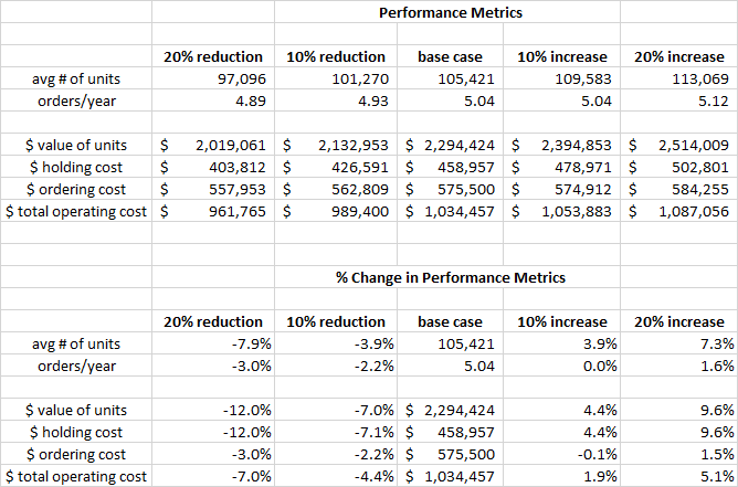
Table 1: Effects of changing lead times

Effect of Order Quantity Restrictions


Table 2 shows the effect of imposing supplier restrictions on order quantities. In the base case, there are no restrictions, i.e., the order minimum is 0 and the order multiple is 1, implying that any order quantity is acceptable to suppliers. Working away from the base case, we first looked at imposing an order minimum of 5 units on all items, then adding an order multiple of 5 for all items.

Forcing orders to be larger than they otherwise would be had the expected impact on the average number of units on hand, increasing it by 0.9% with only an order minimum and by 3.4% with both a minimum and a multiple. The corresponding changes in the dollar value of the inventory were more dramatic: 22.4% and 23.3%. This difference in the size of the percentage response probably traces back to the large number of low-volume/high-cost replacement parts managed by the public transit agency.

Another surprise was the net reduction in operating costs when supplier restrictions were imposed. While holding costs went up by 22.4% and 23.3% in the two what-if scenarios, the larger order quantities allowed for fewer orders per year, resulting in offsetting reductions in ordering costs of, respectively, -24.4% and -32.7%. The net impacts on operating costs were then reductions of 3.7% and 7.9%.

In general, placing restrictions on producer actions would be expected to reduce performance. So the results in these scenarios were counter-intuitive. However, the real message here is that using EOQ, or even enhanced EOQ, to set an order quantity does not give optimum results. Paradoxically, the order quantity restrictions we investigated seem to have forced order quantities closer to optimal levels.


Inventory Optimization - Effect of Order Quantity Restrictions
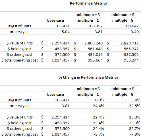
Table 2: Effect of order quantity restrictions

Conclusions


The what-if analyses shown here do not lead to universal conclusions. For instance, changing the assumed cost per order from $40 to some smaller number could show that the supplier restrictions increased rather than decreased the producer’s inventory operating costs.

When doing what-if analysis in real-word situations, users would naturally craft scenarios at a lower level of detail. For instance, they might evaluate the effect of changes in supplier lead times on a supplier-by-supplier basis to find the ones that would have the highest potential payoffs. Or they might arrange for order minima, if they exist already for all items, to change by a specified percentage instead of a fixed amount, which might be somewhat more realistic.

The key takeaway is that inventory optimization software can be used in “what-if mode” to explore strategic issues, beyond its customary use to calculate reorder points, safety stocks, order quantities, and inventory transfers.

Leave a Comment

Related Posts

How to Handle Statistical Forecasts of Zero

How to Handle Statistical Forecasts of Zero

A statistical forecast of zero can cause lots of confusion for forecasters, especially when the historical demand is non-zero. Sure, it’s obvious that demand is trending downward, but should it trend to zero?

Recent Posts

  • The methods of forecasting SoftwareThe Methods of Forecasting
    Demand planning and statistical forecasting software play a pivotal role in effective business management by incorporating features that significantly enhance forecasting accuracy. One key aspect involves the utilization of smoothing-based or extrapolative models, enabling businesses to quickly make predictions based solely on historical data. This foundation rooted in past performance is crucial for understanding trends and patterns, especially in variables like sales or product demand. Forecasting software goes beyond mere data analysis by allowing the blending of professional judgment with statistical forecasts, recognizing that forecasting is not a one-size-fits-all process. This flexibility enables businesses to incorporate human insights and industry knowledge into the forecasting model, ensuring a more nuanced and accurate prediction. […]
  • Learning from Inventory Models Software AILearning from Inventory Models
    In this video blog, the spotlight is on a critical aspect of inventory management: the analysis and interpretation of inventory data. The focus is specifically on a dataset from a public transit agency detailing spare parts for buses. […]
  • Smart Software is in the process of adapting our products to help you cope with your own irregular opsIrregular Operations
    This blog is about “irregular operations.” Smart Software is in the process of adapting our products to help you cope with your own irregular ops. This is a preview. […]
  • Epicor AI Forecasting and Inventory Technology Combined with Planner Knowledge for InsightsSmart Software to Present at Epicor Insights 2024
    Smart Software will present at this year's Epicor Insights event in Nashville. If you plan to attend this year, please join us at booth #13 or #501, and learn more about Epicor Smart Inventory Planning and Optimization. . […]
  • Looking for Trouble in Your Inventory DataLooking for Trouble in Your Inventory Data
    In this video blog, the spotlight is on a critical aspect of inventory management: the analysis and interpretation of inventory data. The focus is specifically on a dataset from a public transit agency detailing spare parts for buses. […]

    Inventory Optimization for Manufacturers, Distributors, and MRO

    • Why MRO Businesses Need Add-on Service Parts Planning & Inventory SoftwareWhy MRO Businesses Need Add-on Service Parts Planning & Inventory Software
      MRO organizations exist in a wide range of industries, including public transit, electrical utilities, wastewater, hydro power, aviation, and mining. To get their work done, MRO professionals use Enterprise Asset Management (EAM) and Enterprise Resource Planning (ERP) systems. These systems are designed to do a lot of jobs. Given their features, cost, and extensive implementation requirements, there is an assumption that EAM and ERP systems can do it all. In this post, we summarize the need for add-on software that addresses specialized analytics for inventory optimization, forecasting, and service parts planning. […]
    • Spare-parts-demand-forecasting-a-different-perspective-for-planning-service-partsThe Forecast Matters, but Maybe Not the Way You Think
      True or false: The forecast doesn't matter to spare parts inventory management. At first glance, this statement seems obviously false. After all, forecasts are crucial for planning stock levels, right? It depends on what you mean by a “forecast”. If you mean an old-school single-number forecast (“demand for item CX218b will be 3 units next week and 6 units the week after”), then no. If you broaden the meaning of forecast to include a probability distribution taking account of uncertainties in both demand and supply, then yes. […]
    • Whyt MRO Businesses Should Care about Excess InventoryWhy MRO Businesses Should Care About Excess Inventory
      Do MRO companies genuinely prioritize reducing excess spare parts inventory? From an organizational standpoint, our experience suggests not necessarily. Boardroom discussions typically revolve around expanding fleets, acquiring new customers, meeting service level agreements (SLAs), modernizing infrastructure, and maximizing uptime. In industries where assets supported by spare parts cost hundreds of millions or generate significant revenue (e.g., mining or oil & gas), the value of the inventory just doesn’t raise any eyebrows, and organizations tend to overlook massive amounts of excessive inventory. […]
    • Top Differences between Inventory Planning for Finished Goods and for MRO and Spare PartsTop Differences Between Inventory Planning for Finished Goods and for MRO and Spare Parts
      In today’s competitive business landscape, companies are constantly seeking ways to improve their operational efficiency and drive increased revenue. Optimizing service parts management is an often-overlooked aspect that can have a significant financial impact. Companies can improve overall efficiency and generate significant financial returns by effectively managing spare parts inventory. This article will explore the economic implications of optimized service parts management and how investing in Inventory Optimization and Demand Planning Software can provide a competitive advantage. […]