
Demand planning and statistical forecasting software play a pivotal role in effective business management by incorporating features that significantly enhance forecasting accuracy. One key aspect involves the utilization of smoothing-based or extrapolative models, enabling businesses to quickly make predictions based solely on historical data. This foundation rooted in past performance is crucial for understanding trends and patterns, especially in variables like sales or product demand. Forecasting software goes beyond mere data analysis by allowing the blending of professional judgment with statistical forecasts, recognizing that forecasting is not a one-size-fits-all process. This flexibility enables businesses to incorporate human insights and industry knowledge into the forecasting model, ensuring a more nuanced and accurate prediction.
Features such as forecasting multiple items as a group, considering promotion-driven demand, and handling intermittent demand patterns are essential capabilities for businesses dealing with diverse product portfolios and dynamic market conditions. Proper implementation of these applications empowers businesses with versatile forecasting tools, contributing significantly to informed decision-making and operational efficiency.
Extrapolative models
Our demand forecasting solutions support a variety of forecasting approaches including extrapolative or smoothing-based forecasting models, such as exponential smoothing and moving averages. The philosophy behind these models is simple: they try to detect, quantify, and project into the future any repeating patterns in the historical data.
There are two types of patterns that might be found in the historical data:
- Trend
- Seasonality
These patterns are illustrated in the following figure along with random data.
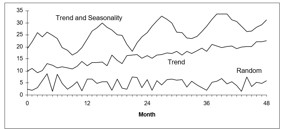
Illustrating trending, seasonal, and random time series data
If the pattern is a trend, then extrapolative models such as double exponential smoothing and linear moving average estimates the rate of increase or decrease in the level of the variable and project that rate into the future.
If the pattern is seasonality, then models such as Winters and triple exponential smoothing estimate either seasonal multipliers or seasonal add factors and then apply these to projections of the nonseasonal portion of the data.
Very often, especially with retail sales data, both trend and seasonal patterns are involved. If these patterns are stable, they can be exploited to give very accurate forecasts.
Sometimes, however, there are no obvious patterns, so that plots of the data look like random noise. Sometimes patterns are clearly visible, but they change over time and cannot be relied upon to repeat. In these cases, the extrapolative models don’t try to quantify and project patterns. Instead, they try to average through the noise and make good estimates of the middle of the distribution of data values. These typical values then become the forecasts. Sometimes, when users see a historical plot with lots of ups and downs they are concerned when the forecast doesn’t replicate those ups and downs. Normally, this should not be a reason for concern. This occurs when the historical patterns aren’t strong enough to warrant using a forecasting method that would replicate the pattern. You want to make sure your forecasts don’t suffer from the “wiggle effect” that is described in this blog post.
Past as a predictor of the future
The key assumption implicit in extrapolative models is that the past is a good guide to the future. This assumption, however, can break down. Some of the historical data may be obsolete. For example, the data might describe a business environment that no longer exists. Or, the world that the model represents may be ready to change soon, rendering all the data obsolete. Because of such complicating factors, the risks of extrapolative forecasting are lower when forecasting only a short time into the future.
Extrapolative models have the practical advantage of being cheap and easy to build, maintain and use. They require only accurate records of past values of the variables you need to forecast. As time goes by, you simply add the latest data points to the time series and reforecast. In contrast, the causal models described below require more thinking and more data. The simplicity of extrapolative models is most appreciated when you have a massive forecasting problem, such as making overnight forecasts of demand for all 30,000 items in inventory in a warehouse.
Judgmental adjustments
Extrapolative models can be run in a fully automatic mode with Demand Planner with no intervention required. Causal models require substantive judgment for wise selection of independent variables. However, both types of statistical models can be enhanced by judgmental adjustments. Both can profit from your insights.
Both causal and extrapolative models are built on historical data. However, you may have additional information that is not reflected in the numbers found in the historical record. For instance, you may know that competitive conditions will soon change, perhaps due to price discounts, or industry trends, or the emergence of new competitors, or the announcement of a new generation of your own products. If these events occur during the period for which you are forecasting, they may well spoil the accuracy of purely statistical forecasts. Smart Demand Planner’ graphical adjustment feature lets you include these additional factors in your forecasts through the process of on- screen graphical adjustment.
Be aware that applying user adjustments to the forecast is a two-edged sword. Used appropriately, it can enhance forecast accuracy by exploiting a richer set of information. Used promiscuously, it can add additional noise to the process and reduce accuracy. We advise that you use judgmental adjustments sparingly, but that you never blindly accept the predictions of a purely statistical forecasting method. It is also very important to measure forecast value add. That is, the value added to the forecast process by each incremental step. For example, if you are applying overrides based on business knowledge, it is important to measure whether those adjustments are adding value by improving forecast accuracy. Smart Demand Planner supports measurement of forecast value add by tracking every forecast considered and automating the forecast accuracy reports. You can select statistical forecasts, measure their errors, and compare them to the overridden ones. By doing so, you inform the forecasting process so that better decisions can be made in the future.
Multiple-level forecasts
Another common situation involves multiple-level forecasting, where there are multiple items being forecast as a group or there may even be multiple groups, with each group containing multiple items. We will generally call this type of forecasting Multilevel Forecasting. The prime example is product line forecasting, where each item is a member of a family of items, and the total of all the items in the family is a meaningful quantity.
For example, as in the following figure, you might have a line of tractors and want forecasts of sales for each type of tractor and for the entire tractor line.
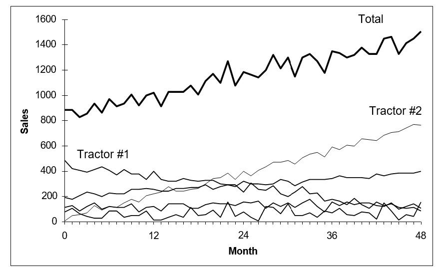
Illustrating multiple-level product forecasts
Smart Demand Planner provides Roll Up/Roll Down Forecasting. This function is crucial for obtaining comprehensive forecasts of all product items and their group total. The Roll Down/Roll Up method within this feature offers two options for obtaining these forecasts:
Roll Up (Bottom-Up): This option initially forecasts each item individually and then aggregates the item-level forecasts to generate a family-level forecast.
Roll Down (Top-Down): Alternatively, the roll-down option starts by forming the historical total at the family level, forecasts it, and then proportionally allocates the total down to the item level.
When utilizing Roll Down/Roll Up, you have access to the full array of forecast methods provided by Smart Demand Planner at both the item and family levels. This ensures flexibility and accuracy in forecasting, catering to the specific needs of your business across different hierarchical levels.
Forecasting research has not established clear conditions favoring either the top-down or bottom-up approach to forecasting. However, the bottom-up approach seems preferable when item histories are stable, and the emphasis is on the trends and seasonal patterns of the individual items. Top-down is normally a better choice if some items have very noisy history or the emphasis is on forecasting at the group level. Since Smart Demand Planner makes it fast and easy to try both a bottom-up and a top- down approach, you should try both methods and compare the results. You can use Smart Demand Planner’s “Hold back on Current” feature in the “Forecast vs. Actual” to test both approaches on your own data and see which one yields a more accurate forecast for your business.