Here are examples of forecasting problems that SmartForecasts can solve, along with the kinds of business data representative of each.

Forecasting an item based on its pattern

Given the following six quarterly sales figures, what sales can you expect for the third and fourth quarters of 2023?

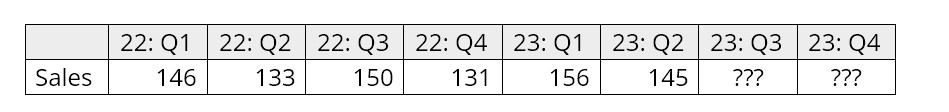
Sales by Quarter

SmartForecasts gives you many ways to approach this problem. You can make your own statistical forecasts using any of six different exponential smoothing and moving average methods. Or, like most nontechnical forecasters, you can use the time-saving Automatic command, which has been programmed to automatically select and use the most accurate method for your data. Finally, to incorporate your business judgment into the forecasting process, you can graphically adjust any statistical forecast result using SmartForecasts’ “eyeball” adjustment capabilities.

Forecasting an item based on its relationship to other variables.

Given the following historical relationship between unit sales and the number of sales representatives, what sales levels can you expect when the planned increase in sales staff takes place over the final two quarters of 2023?

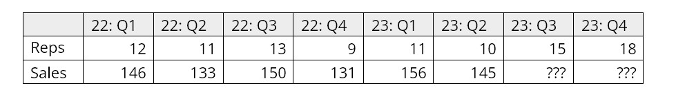
Sales and Sales Representatives by Quarter

You can answer a question like this using SmartForecasts’ powerful Regression command, designed specifically to facilitate forecasting applications that require regression analysis solutions. Regression models with an essentially unlimited number of independent/predictor variables are possible, although most useful regression models use only a handful of predictors.

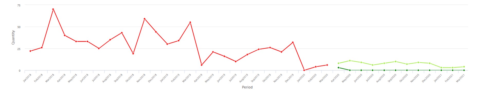
Simultaneously forecasting a number of product items and their total

Given the following total sales for all dress shirts and the distribution of sales by color, what will individual and total sales be over the next six months?

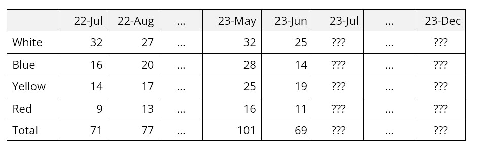
Monthly Dress Shirt Sales by Color

SmartForecasts’ unique Group Forecasting features automatically and simultaneously forecasts closely related time series, such as these items in the same product group. This saves considerable time and provides forecast results not only for the individual items but also for their total. “Eyeball” adjustments at both the item and group levels are easy to make. You can quickly create forecasts for product groups with hundreds or even thousands of items.

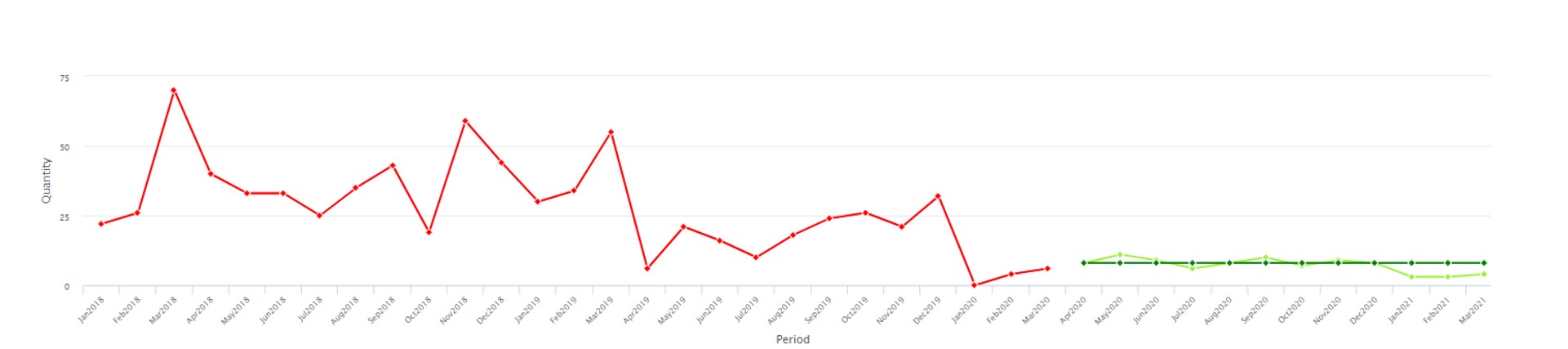
Forecasting thousands of items automatically

Given the following record of product demand at the SKU level, what can you expect demand to be over the next six months for each of the 5,000 SKUs?

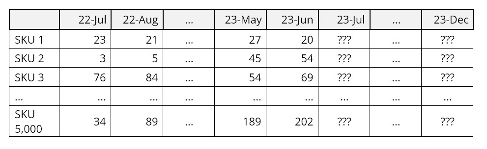
Monthly Product Demand by SKU (Stock Keeping Unit)

In just a few minutes, SmartForecasts’ powerful Automatic Selection can take a forecasting job of this size, read the product demand data, automatically create statistical forecasts for each SKU, and saves the result. The results are then ready for export to your ERP system leveraging any one of our API-based connectors or via file export.  Once set up, forecasts will automatically be produced each planning cycle without intervention by the user.

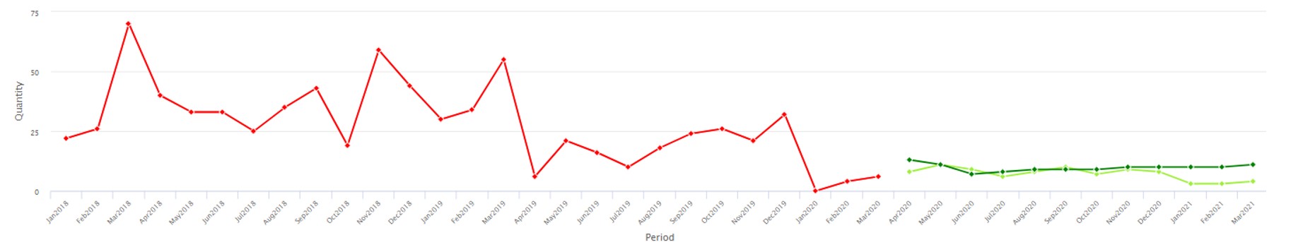
Forecasting demand that is most often zero

A distinct and especially challenging type of data to forecast is intermittent demand, which is most often zero but jumps up to random nonzero values at random times. This pattern is typical of demand for slow moving items, such as service parts or big ticket capital goods.

For example, consider the following sample of demand for aircraft service parts. Note the preponderance of zero values with nonzero values mixed in, often in bursts.

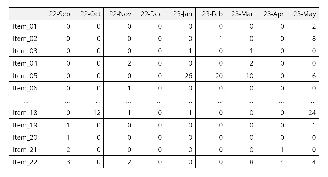
SmartForecasts has a unique method designed especially for this type of data: the Intermittent Demand forecasting feature. Since intermittent demand arises most often in the context of inventory control, this feature focuses on forecasting the range of likely values for the total demand over a lead time, e.g., cumulative demand over the period Jun-23 to Aug-23 in the example above.

Forecasting inventory requirements

Forecasting inventory requirements is a specialized variant of forecasting that focuses on the high end of the range of possible future values.

For simplicity, consider the problem of forecasting inventory requirements for just one period ahead, say one day ahead. Usually, the forecasting job is to estimate the most likely or average level of product demand. However, if available inventory equals the average demand, there is about a 50% chance that demand will exceed inventory, resulting in lost sales and/or lost good will. Setting the inventory level at, say, ten times the average demand will probably eliminate the problem of stockouts, but will just as surely result in bloated inventory costs.

The trick of inventory optimization is to find a satisfactory balance between having enough inventory to meet most demand without tying up too many resources in the process. Usually, the solution is a blend of business judgment and statistics. The judgmental part is to define an acceptable inventory service level, such as meeting 95% of demand immediately from stock. The statistical part is to estimate the 95th percentile of demand.

When not dealing with intermittent demand, SmartForecasts estimates the required inventory level by assuming a bell-shaped (Normal) curve of demand, estimating both the middle and the width of the bell curve, then using a standard statistical formula to estimate the desired percentile. The difference between the desired inventory level and the average level of demand is called the safety stock because it protects against the possibility of stockouts.

When dealing with intermittent demand, the bell-shaped curve is a poor approximation to the statistical distribution of demand. In this special case, SmartForecasts uses patented intermittent demand forecasting technology to estimate the required inventory service level.

Forecast accuracy is a key metric by which to judge the quality of your demand planning process. (It’s not the only one. Others include timeliness and cost; See 5 Demand Planning Tips for Calculating Forecast Uncertainty.) Once you have forecasts, there are a number of ways to summarize their accuracy, usually designated by obscure three- or four-letter acronyms like MAPE, RMSE, and MAE.  See Four Useful Ways to Measure Forecast Error for more detail.

A less discussed but more fundamental issue is how computational experiments are organized for computing forecast error. This post compares the three most important experimental designs. One of them is old-school and essentially amounts to cheating. Another is the gold standard. A third is a useful expedient that mimics the gold standard and is best thought of as predicting how the gold standard will turn out. Figure 1 is a schematic view of the three methods.

Figure 1: Three ways to assess forecast error

The top panel of Figure 1 depicts the way forecast error was assessed back in the early 1980’s before we moved the state of the art to the scheme shown in the middle panel. In the old days, forecasts were assessed on the same data used to compute the forecasts. After a model was fit to the data, the errors computed were not for model forecasts but for model fits. The difference is that forecasts are for future values, while fits are for concurrent values. For example, suppose the forecasting model is a simple moving average of the three most recent observations. At time 3, the model computes the average of observations 1, 2, and 3. This average would then be compared to the observed value at time 3. We call this cheating because the observed value at time 3 got a vote on what the forecast should be at time 3. A true forecast assessment would compare the average of the first three observations to the value of the next, fourth, observation. Otherwise, the forecaster is left with an overly optimistic assessment of forecast accuracy.

The bottom panel of Figure 1 shows the best way to assess forecast accuracy. In this schema, all the historical demand data are used to fit a model, which is then used to forecast future, unknown demand values. Eventually, the future unfolds, the true future values reveal themselves, and actual forecast errors can be computed. This is the gold standard. This information populates the “forecasts versus actuals” report in our software.

The middle panel depicts a useful halfway measure. The problem with the gold standard is that you must wait to learn how well your chosen forecasting methods perform. This delay does not help when you are required to choose, in the moment, which forecasting method to use for each item. Nor does it provide a timely estimate of the forecast uncertainty you will experience, which is important for risk management such as forecast hedging. The middle way is based on hold-out analysis, which excludes (“holds out”) the most recent observations and asks the forecasting method to do its work without knowing those ground truths. Then the forecasts based on the foreshortened demand history can be compared to the held-out actual values to get an honest assessment of forecast error.

In a recent LinkedIn post, I detailed four questions that, when answered, will reveal how forecasts are being used in your business.  In this article, we’ve listed questions you can ask that will reveal how forecasts are created.

1. When we ask users how they create forecasts, their answer will often be “we use history.” This obviously isn’t enough information, as there are different types of demand history that require different forecasting methods. If you are using historical data, then make sure to find out if you are using an averaging model, a trending model, a seasonal model, or something else to forecast.

2. Once you know the model used, ask about the parameter values of those models. The forecast output of an “average” will differ, sometimes significantly, depending on the number of periods you are averaging.  So, find out whether you are using an average of the last 3 months, 6 months, 12 months, etc.

3. If you are using trending models, ask how the model weights are set. For example, in a trending model, such as double exponential smoothing, the forecasts will differ significantly depending on how the calculations weight recent data compared to older data (higher weights put more emphasis on the recent data).

4. If you are using seasonal models, the forecast results are going to be impacted by the “level” and “trending weights” used. You should also determine whether seasonal periods are forecasted with multiplicative or additive seasonality.  (Additive seasonality says, e.g., “Add 100 units for July”, whereas multiplicative seasonality says “Multiply by 1.25 for July.”) Finally, you may not be using these types of methods at all.  Some practitioners will use a forecast method that simply averages prior periods (i.e., next June will be forecasted based on the average of the prior three Junes).

5. How do you go about choosing one model over another? Does the choice of technique depend on the type of demand data or when new demand data are available? Is this process automated? Or if a planner chooses a trend model subjectively, will that item continue to be forecasted with that model until the planner changes it again?

6. Are your forecasts “fully automatic,” so that trend and/or seasonality are detected automatically? Or are your forecasts dependent on item classifications that must be maintained by users? The latter requires more time and attention from planners to define what behavior constitutes trend, seasonality, etc.

7. What are the item classification rules used? For example, an item may be considered a trending item if demand increases by more than 5% period-over-period. An item may be considered seasonal if 70% or more of the annual demand occurs in four or fewer periods. Such rules are user-defined and often require overly broad assumptions. Sometimes they are configured when a system was originally implemented but never revised even as conditions change. It’s important to make sure any classification rules are understood and, if necessary, updated.

8. Does the forecast regenerate automatically when new data are available, or do you have to manually regenerate the forecasts?

9. Do you check for any change in forecast from one period to the next before deciding whether to use the new forecast? Or do you default to the new forecast?

10. How are forecast overrides that were made in prior planning cycles treated when a new forecast is created? Are they reused or replaced?

11. How do you incorporate forecasts made by your sales team or by your customers? Do these forecasts replace the baseline forecast, or do you use these inputs to make planner overrides to the baseline forecast?

12. Under what circumstances would you ignore the baseline forecast and use exactly what sales or customers are telling you?

13. If you rely on customer forecasts, what do you do about customers who don’t provide forecasts?

14. How do you document the effectiveness of your forecasting approach?  Most companies only measure the accuracy of the final forecast that is submitted to the ERP system, if they measure anything. But they don’t assess alternative predictions that might have been used. It is important to compare what you are doing to benchmarks. For example, do the methods you are using outperform a naïve forecast (i.e., “tomorrow equals today,” which requires no thought), or what you saw last year, or the average of the last 12 months.  Benchmarking your baseline forecast insures you are squeezing as much accuracy as possible out of the data.

15. Do you measure whether overrides from sales, customers, and planners are making the forecast better or worse? This is just as important as measuring whether your statistical approaches are outperforming the naïve method.  If you don’t know whether overrides are helping or hurting, the business can’t get better at forecasting – you need to know which steps are adding value so that you can do more of those and get even better. If you aren’t documenting forecast accuracy and conducting “forecast value add” analysis, then you aren’t able to properly assess whether the forecasts being produced are the best you could make.  You’ll miss opportunities to improve the process, increase accuracy, and educate the business on what type of forecast error is to be expected.

Smart IP&O is powered by the SmartForecasts® forecasting engine that automatically selects the most appropriate method for each item.  Smart Forecast methods are listed below:

• Simple Moving Average and Single Exponential Smoothing for flat, noisy data
• Linear Moving Average and Double Exponential Smoothing for trending data
• Winters Additive and Winters Multiplicative for seasonal and seasonal & trending data.

This blog explains how each model works using time plots of historical and forecast data.  It outlines how to go about choosing which model to use.   The examples below show the same history, in red, forecasted with each method, in dark green, compared to the Smart-chosen winning method, in light green.

Seasonality
If you want to force (or prevent) seasonality to show in the forecast, then choose Winters models.  Both methods require 2 full years of history.

`Winter’s multiplicative will determine the size of the peaks or valleys of seasonal effects based on a percentage difference from a trending average volume.  It is not a good fit for very low volume items due to division by zero when determining that percentage. Note in the image below that the large percentage drop in seasonal demand in the history is being projected to continue over the forecast horizon making it look like there isn’t any seasonal demand despite using a seasonal method.

Statistical forecast produced with Winter’s multiplicative method. 

Winter’s additive will determine the size of the peaks or valleys of seasonal effects based on a unit difference from the average volume.  It is not a good fit if there’s significant trend to the data.  Note in the image below that seasonality is now being forecasted based on the average unit change in seasonality. So, the forecast still clearly reflects the seasonal pattern despite the down trend in both the level and seasonal peaks/valleys.

Statistical forecast produced with Winter’s additive method.

Trend

If you want to force (or prevent) trend up or down to show in the forecast, then restrict the chosen methods to (or remove the methods of) Linear Moving Average and Double Exponential Smoothing.

 Double exponential smoothing will pick up on a long-term trend.  It is not a good fit if there are few historical data points.

Statistical forecast produced with Double Exponential Smoothing

Linear moving average will pick up on nearer term trends.  It is not a good fit for highly volatile data

Non-Trending and Non-Seasonal Data
If you want to force (or prevent) an average from showing in the forecast, then restrict the chosen methods to (or remove the methods of) Simple Moving Average and Single Exponential Smoothing.

Single exponential smoothing will weigh the most recent data more heavily and produce a flat-line forecast.  It is not a good fit for trending or seasonal data.

Statistical forecast using Single Exponential Smoothing

Simple moving average will find an average for each period, sometimes appearing to wiggle, and better for longer-term averaging.  It is not a good fit for trending or seasonal data.

Statistical forecast using Simple Moving Average

Sometimes a statistical forecast just doesn’t make sense.  Every forecaster has been there.  They may double-check that the data was input correctly or review the model settings but are still left scratching their head over why the forecast looks very unlike the demand history.   When the occasional forecast doesn’t make sense, it can erode confidence in the entire statistical forecasting process.

This blog will help a layman understand what the Smart statistical models are and how they are chosen automatically.  It will address how that choice sometimes fails, how you can know if it did, and what you can do to ensure that the forecasts can always be justified.  It’s important to know to expect, and how to catch the exceptions so you can rely on your forecasting system.

How methods are chosen automatically

The criteria to automatically choose one statistical method out of a set is based on which method came closest to correctly predicting held-out history.  Earlier history is passed to each method and the result is compared to actuals to find the one that came closest overall.  That automatically chosen method is then fed all the history to produce the forecast. Check out this blog to learn more about the model selection https://smartcorp.com/uncategorized/statistical-forecasting-how-automatic-method-selection-works/

For most time series, this process can capture trends, seasonality, and average volume accurately. But sometimes a chosen method comes mathematically closest to predicting the held-out history but doesn’t project it forward in a way that makes sense.  That means the system selected method isn’t best and for some “hard to forecast”

Hard to forecast items

Hard to forecast items may have large, unpredictable spikes in demand, or typically no demand but random irregular blips, or unusual recent activity.  Noise in the data sometimes randomly wanders up or down, and the automated best-pick method might forecast a runaway trend or a grind into zero.  It will do worse than common sense and in a small percentage of any reasonably varied group of items.  So, you will need to identify these cases and respond by overriding the forecast or changing the forecast inputs.

How to find the exceptions

Best practice is to filter or sort the forecasted items to identify those where the sum of the forecast over the next year is significantly different than the corresponding history last year.  The forecast sum may be much lower than the history or vice versa.  Use supplied metrics to identify these items; then you can choose to apply overrides to the forecast or modify the forecast settings.

How to fix the exceptions

Often when the forecast seems odd, an averaging method, like Single Exponential Smoothing or even a simple average using Freestyle, will produce a more reasonable forecast.  If trend is possibly valid, you can remove only seasonal methods to avoid a falsely seasonal result.  Or do the opposite and use only seasonal methods if seasonality is expected but wasn’t projected in the default forecast.  You can use the what-if features to create any number of forecasts, evaluate & compare, and continue to fine tune the settings until you are comfortable with the forecast.

Cleaning the history, with or without changing the automatic method selection, is also effective at producing reasonable forecasts. You can embed forecast parameters to reduce the amount of history used to forecast those items or the number of periods passed into the algorithm so earlier, outdated history is no longer considered.  You can edit spikes or drops in the demand history that are known anomalies so they don’t influence the outcome.  You can also work with the Smart team to implement automatic outlier detection and removal so that data prior to being forecasted is already cleansed of these anomalies.

If the demand is truly intermittent, it is going to be nearly impossible to forecast “accurately” per period. If a level-loading average is not acceptable, handling the item by setting inventory policy with a lead time forecast can be effective.  Alternatively, you may choose to use “same as last year” models which while not prone to accuracy will be generally accepted by the business given the alternatives forecasts.

Finally, if the item was introduced so recently that the algorithms do not have enough input to accurately forecast, a simple average or manual forecast may be best.  You can identify new items by filtering on the number of historical periods.

Manual selection of methods

Once you have identified rows where the forecast doesn’t make sense to the human eye, you can choose a smaller subset of all methods to allow into the forecast run and compare to history.  Smart will allow you to use a restricted set of methods just for one forecast run or embed the restricted set to use for all forecast runs going forward. Different methods will project the history into the future in different ways.  Having a sense of how each works will help you choose which to allow.

Rely on your forecasting tool

The more you use Smart period over period to embed your decisions about how to forecast and what historical data to consider, the less often you will face exceptions as described in this blog.  Entering forecast parameters is a manageable task when starting with critical or high impact items.  Even if you don’t embed any manual decisions on forecast methods, the forecast re-runs every period with new data. So, an item with an odd result today can become easily forecastable in time.