Outside of work, you may have heard the famous dictum “Correlation is not causation.” It may sound like a piece of theoretical fluff that, though involved in a recent Noble Prize in economics, isn’t relevant to your work as a demand planner. Is so, you may be only partially correct.

Extrapolative vs Causal Models

Most demand forecasting uses extrapolative models. Also called time-series models, these forecast demand using only the past values of an item’s demand. Plots of past values reveal trend and seasonality and volatility, so there is a lot they are good for. But there is another type of model – causal models —that can potentially improve forecast accuracy beyond what you can get from extrapolative models.

Causal models bring more input data to the forecasting task: information on presumed forecast “drivers” external to the demand history of an item. Examples of potentially useful causal factors include macroeconomic variables like the inflation rate, the rate of GDP growth, and raw material prices. Examples not tied to the national economy include industry-specific growth rates and your own and competitors’ ad spending.  These variables are usually used as inputs to regression models, which are equations with demand as an output and causal variables as inputs.

Forecasting using Causal Models

Many firms have an S&OP process that involves a monthly review of statistical (extrapolative) forecasts in which management adjusts forecasts based on their judgement. Often this is an indirect and subjective way to work causal models into the process without doing the regression modeling.

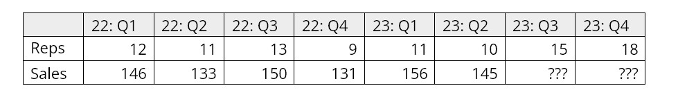
To actually make a causal regression model, first you have to nominate a list of potentially-useful causal predictor variables. These may come from your subject matter expertise. For example, suppose you manufacture window glass. Much of your glass may end up in new homes and new office buildings. So, the number of new homes and offices being built are plausible predictor variables in a regression equation.

There is a complication here: if you are using the equation to predict something, you must first predict the predictors. For example, sales of glass next quarter may be strongly related to numbers of new homes and new office buildings next quarter. But how many new homes will there be next quarter? That’s its own forecasting problem. So, you have a potentially powerful forecasting model, but you have extra work to do to make it usable.

There is one way to simplify things: if the predictor variables are “lagged” versions of themselves. For example, the number of new building permits issued six months ago may be a good predictor of glass sales next month. You don’t have to predict the building permit data – you just have to look it up.

Is it a causal relationship or just a spurious correlation?

Causal models are the real deal: there is an actual mechanism that relates the predictor variable to the predicted variable. The example of predicting glass sales from building permits is an example.

A correlation relationship is more iffy. There is a statistical association that may or may not provide a solid basis for forecasting. For example, suppose you sell a product that happens to appeal most strongly to Dutch people but you don’t realize this. The Dutch are, on average, the tallest people in Europe. If your sales are increasing and the average height of Europeans is increasing, you might use that relationship to good effect. However, if the proportion of Dutch in the Euro zone is decreasing while the average height is increasing because the mix of men versus women is shifting toward men, what can go wrong? You will expect sales to increase because average height is increasing. But your sales are really mostly to the Dutch, and their relative share of the population is shrinking, so your sales are really going to decrease instead. In this case the association between sales and customer height is a spurious correlation.

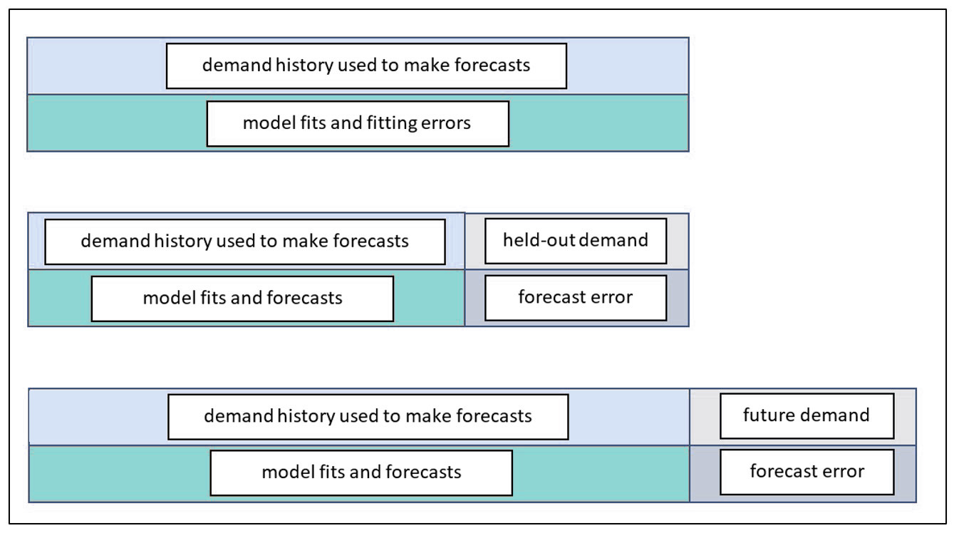
How can you tell the difference between true and spurious relationships? The gold standard is to do a rigorous scientific experiment. But you are not likely to be in position to do that. Instead, you have to rely on your personal “mental model” of how your market works. If your hunches are right, then your potential causal models will correlate with demand and causal modeling will pay off for you, either to supplement extrapolative models or to replace them.

Here are examples of forecasting problems that SmartForecasts can solve, along with the kinds of business data representative of each.

Forecasting an item based on its pattern

Given the following six quarterly sales figures, what sales can you expect for the third and fourth quarters of 2023?

Sales by Quarter

SmartForecasts gives you many ways to approach this problem. You can make your own statistical forecasts using any of six different exponential smoothing and moving average methods. Or, like most nontechnical forecasters, you can use the time-saving Automatic command, which has been programmed to automatically select and use the most accurate method for your data. Finally, to incorporate your business judgment into the forecasting process, you can graphically adjust any statistical forecast result using SmartForecasts’ “eyeball” adjustment capabilities.

Forecasting an item based on its relationship to other variables.

Given the following historical relationship between unit sales and the number of sales representatives, what sales levels can you expect when the planned increase in sales staff takes place over the final two quarters of 2023?

Sales and Sales Representatives by Quarter

You can answer a question like this using SmartForecasts’ powerful Regression command, designed specifically to facilitate forecasting applications that require regression analysis solutions. Regression models with an essentially unlimited number of independent/predictor variables are possible, although most useful regression models use only a handful of predictors.

Simultaneously forecasting a number of product items and their total

Given the following total sales for all dress shirts and the distribution of sales by color, what will individual and total sales be over the next six months?

Monthly Dress Shirt Sales by Color

SmartForecasts’ unique Group Forecasting features automatically and simultaneously forecasts closely related time series, such as these items in the same product group. This saves considerable time and provides forecast results not only for the individual items but also for their total. “Eyeball” adjustments at both the item and group levels are easy to make. You can quickly create forecasts for product groups with hundreds or even thousands of items.

Forecasting thousands of items automatically

Given the following record of product demand at the SKU level, what can you expect demand to be over the next six months for each of the 5,000 SKUs?

Monthly Product Demand by SKU (Stock Keeping Unit)

In just a few minutes, SmartForecasts’ powerful Automatic Selection can take a forecasting job of this size, read the product demand data, automatically create statistical forecasts for each SKU, and saves the result. The results are then ready for export to your ERP system leveraging any one of our API-based connectors or via file export.  Once set up, forecasts will automatically be produced each planning cycle without intervention by the user.

Forecasting demand that is most often zero

A distinct and especially challenging type of data to forecast is intermittent demand, which is most often zero but jumps up to random nonzero values at random times. This pattern is typical of demand for slow moving items, such as service parts or big ticket capital goods.

For example, consider the following sample of demand for aircraft service parts. Note the preponderance of zero values with nonzero values mixed in, often in bursts.

SmartForecasts has a unique method designed especially for this type of data: the Intermittent Demand forecasting feature. Since intermittent demand arises most often in the context of inventory control, this feature focuses on forecasting the range of likely values for the total demand over a lead time, e.g., cumulative demand over the period Jun-23 to Aug-23 in the example above.

Forecasting inventory requirements

Forecasting inventory requirements is a specialized variant of forecasting that focuses on the high end of the range of possible future values.

For simplicity, consider the problem of forecasting inventory requirements for just one period ahead, say one day ahead. Usually, the forecasting job is to estimate the most likely or average level of product demand. However, if available inventory equals the average demand, there is about a 50% chance that demand will exceed inventory, resulting in lost sales and/or lost good will. Setting the inventory level at, say, ten times the average demand will probably eliminate the problem of stockouts, but will just as surely result in bloated inventory costs.

The trick of inventory optimization is to find a satisfactory balance between having enough inventory to meet most demand without tying up too many resources in the process. Usually, the solution is a blend of business judgment and statistics. The judgmental part is to define an acceptable inventory service level, such as meeting 95% of demand immediately from stock. The statistical part is to estimate the 95th percentile of demand.

When not dealing with intermittent demand, SmartForecasts estimates the required inventory level by assuming a bell-shaped (Normal) curve of demand, estimating both the middle and the width of the bell curve, then using a standard statistical formula to estimate the desired percentile. The difference between the desired inventory level and the average level of demand is called the safety stock because it protects against the possibility of stockouts.

When dealing with intermittent demand, the bell-shaped curve is a poor approximation to the statistical distribution of demand. In this special case, SmartForecasts uses patented intermittent demand forecasting technology to estimate the required inventory service level.

Forecast accuracy is a key metric by which to judge the quality of your demand planning process. (It’s not the only one. Others include timeliness and cost; See 5 Demand Planning Tips for Calculating Forecast Uncertainty.) Once you have forecasts, there are a number of ways to summarize their accuracy, usually designated by obscure three- or four-letter acronyms like MAPE, RMSE, and MAE.  See Four Useful Ways to Measure Forecast Error for more detail.

A less discussed but more fundamental issue is how computational experiments are organized for computing forecast error. This post compares the three most important experimental designs. One of them is old-school and essentially amounts to cheating. Another is the gold standard. A third is a useful expedient that mimics the gold standard and is best thought of as predicting how the gold standard will turn out. Figure 1 is a schematic view of the three methods.

Figure 1: Three ways to assess forecast error

The top panel of Figure 1 depicts the way forecast error was assessed back in the early 1980’s before we moved the state of the art to the scheme shown in the middle panel. In the old days, forecasts were assessed on the same data used to compute the forecasts. After a model was fit to the data, the errors computed were not for model forecasts but for model fits. The difference is that forecasts are for future values, while fits are for concurrent values. For example, suppose the forecasting model is a simple moving average of the three most recent observations. At time 3, the model computes the average of observations 1, 2, and 3. This average would then be compared to the observed value at time 3. We call this cheating because the observed value at time 3 got a vote on what the forecast should be at time 3. A true forecast assessment would compare the average of the first three observations to the value of the next, fourth, observation. Otherwise, the forecaster is left with an overly optimistic assessment of forecast accuracy.

The bottom panel of Figure 1 shows the best way to assess forecast accuracy. In this schema, all the historical demand data are used to fit a model, which is then used to forecast future, unknown demand values. Eventually, the future unfolds, the true future values reveal themselves, and actual forecast errors can be computed. This is the gold standard. This information populates the “forecasts versus actuals” report in our software.

The middle panel depicts a useful halfway measure. The problem with the gold standard is that you must wait to learn how well your chosen forecasting methods perform. This delay does not help when you are required to choose, in the moment, which forecasting method to use for each item. Nor does it provide a timely estimate of the forecast uncertainty you will experience, which is important for risk management such as forecast hedging. The middle way is based on hold-out analysis, which excludes (“holds out”) the most recent observations and asks the forecasting method to do its work without knowing those ground truths. Then the forecasts based on the foreshortened demand history can be compared to the held-out actual values to get an honest assessment of forecast error.

“Despite what you’ve seen in your Saturday morning cartoons, elephants can’t jump, and there’s one simple reason: They don’t have to. Most jumpy animals—your kangaroos, monkeys, and frogs—do it primarily to get away from predators.”  — Patrick Monahan, Science.org, Jan 27, 2016.

Now you know why the largest ERP companies can’t develop high quality best-of-breed like solutions. They never had to, so they never evolved to innovate outside of their core focus. 

However, as ERP systems have become commoditized, gaps in their functionality became impossible to ignore. The larger players sought to protect their share of customer wallet by promising to develop innovative add-on applications to fill all the white spaces.  But without that “innovation muscle,” many projects failed, and mountains of technical debt accumulated.

Best-of-breed companies evolved to innovate and have deep functional expertise in specific verticals.  The result is that best of breed ERP add-ons are easier to use, have more features, and deliver more value than the native ERP modules they replace. 

If your ERP provider has already partnered with an innovative best of breed add-on provider*, you’re all set! But if you can only get the basics from your ERP, go with a best-of-breed add-on that has a bespoke integration to the ERP. 

A great place to start your search is to look for ERP demand planning add-ons that add brains to the ERP’s brawn, i.e., those that support inventory optimization and demand forecasting.  Leverage add-on tools like Smart’s statistical forecasting, demand planning, and inventory optimization apps to develop forecasts and stocking policies that are fed back to the ERP system to drive daily ordering. 

*App-stores are a license for the best of breed to sell into the ERP companies base –  being listed  partnerships.

There’s one thing I’m reminded of almost every day at Smart Software that puzzle me: most companies do not understand how forecasts are created, and stocking policies are determined.  It’s an organizational black box. Here is an example from a recent sales call:

How do you forecast?
We use history.

How do you use history?
What do you mean?

Well, you can take an average of the last year, last two years, average the most recent periods, or use some other type of formula to generate the forecast.
I’m pretty sure we use an average of the last 12 months.

Why 12 months instead of a different amount of history?
12 months is a good amount of time to use because it doesn’t get skewed by older data but it’s recent enough

How do you know it’s more accurate than using 18 months or some other length of history?
We don’t know. We do adjust the forecasts based on feedback from sales.  

Do you know if the adjustments make things more accurate or less than if you just used the average?
We don’t know but are confident that forecasts are inflated

What do the inventory buyers do then if they think the numbers are inflated?
They have lots of business knowledge and adjust their buys accordingly

So, is it fair to say they would ignore the forecasts at least some of the time?
Yes, some of the time.

How do the buyers decide when to order more? Do you have a reorder point or safety stock specified in your ERP system that helps guide these decisions?
Yes, we use a safety stock field.

How is safety stock calculated?
Buyers determine this based on the importance of the item, lead times, and other considerations such as how many customers purchase the item, the velocity of the item, it’s cost.  They’ll carry different amounts of safety stock depending on this.

The discussion continued. The main takeaway here is that when you scratch just below the surface, far more questions are revealed than answers.  This often means that the inventory planning and demand forecast process is highly subjective, varies from planner to planner, is not well understood by the rest of the organization, and likely to be reactive.  As Tom Willemain has described it’s “chaos masked by improvisation.”   The “as-is” process needs to be fully identified and documented.  Only then can gaps be exposed, and improvements can be made.   Here is a list of 10 questions  you can ask that will reveal your organization’s true forecasting, demand planning, and inventory planning process.