In a previous post, I discussed one of the thornier problems demand planners sometimes face: working with product demand data characterized by what statisticians call skewness — a situation that can necessitate costly inventory investments. This sort of problematic data is found in several different scenarios. In at least one, the combination of intermittent demand and very effective sales promotions, the problem lends itself to an effective solution.

Reviewing terms, recall that “service level” is the probability of not stocking out while waiting for a replenishment order to arrive, while “fill rate” is the percentage of demand that is satisfied immediately from stock. In my previous post, “The Scourge of Skewness”, I pointed out that a certain type of demand distribution, having a “long right tail”, will lead to fill rates that can be much lower than service levels. I also pointed out that sometimes the only way to improve the fill rate is to increase the target service level to an unusually high level, which can be expensive.

In this post, I’ll look at solving the problem in one special case: skewness resulting from effective sales promotions mixed with “intermittent demand”. Intermittent demand has a large proportion of zero values, with nonzero values mixed in at random. Successful sales promotions, obviously positive, have a downside: they can confuse the “demand signal” with spikes in your demand history, and can undermine forecasts and bias safety stock calculations. When intermittent demand and effective sales promotions are the source of your data’s skewness, methods exist to work around the problem to achieve both higher fill rates and more accurate demand forecasts.

How Promotions Increase Skewness

Successful promotions abruptly increase item demand. This creates anomalies, or “outliers”, which contribute to forming a skewed distribution. Knowing when promotions occurred in the past, we can adjust an item’s record of past demand. We produce an alternate demand history as if there had been no promotions, by replacing the outliers with values more representative of the “natural” level of demand. These adjustments reduce demand skewness. Reduced skewness can lead to significant reductions in both expected forecasts and safety stocks, which add together to form reorder points.

Successful promotions are likely to be repeated. When that happens, the promotion effects can be added in to demand forecasts to increase their accuracy. The effect of future promotions on inventory management will be to increase the risk of stockouts, so a sensible response is to work at the operational level to build up temporary supply, in a quantity keyed to the estimated impact of prior promotions on the effected items.

Using Event Modeling to Improve Demand Forecasting

It’s possible to model the impact of like events, and apply this to planned events in the future. Doing so can improve your forecast in two big ways: by projecting the demand jolt you expect from a planned event; and rationalizing the spikes in the past that were caused by events, making your baseline activity more visible and more accurately forecastable. We do a lot of this in SmartForecasts, so allow me to use our experience there to show you what I mean.

Event Modeling entails the following steps:
• Automatically estimating the impact of previous promotions (which is a useful result in itself).
• Adjusting historical demand to statistically remove the effect of promotions.
• Creating promotion-free forecasts.
• Revising the forecasts for any future time periods in which promotions are planned.

We call this this type of analysis “Promo forecasting”. We use the word “promotions” to describe what you do yourself to improve your results. We use “events” to describe what the world does to you, usually to your detriment; examples include strikes, power outages, warehouse fires and other unlucky happenings.

To understand how Event Modeling can help you cope with skewness when doing demand forecasting for high-volume items, consider Figures 1-3.

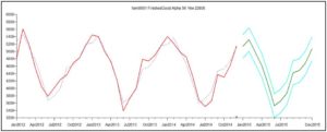
Figure 1 shows that this item’s demand pattern is clearly seasonal, and the forecast is both seasonal and “tight”, meaning that the forecast uncertainty interval (“margin of error”, shown in cyan lines) is very narrow.

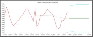
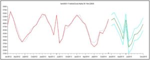
Figure 2 shows an alternative history in which a promotion in June 2014 reversed the usual seasonal low associated with June sales. This demand pattern was forecasted using the Automatic forecasting tournament in SmartForecasts, as in Figure 1. This time, the promotion scrambled the seasonal pattern enough to create an inappropriate non-seasonal forecast, and one that has a much larger margin of error.

Finally, Figure 3 shows how Promo forecasting handles the same promoted scenario, retaining a seasonal forecast and building into the forecast an estimate of the effect of a planned repeat promotion in 2015.

The Case of Intermittent Demand

In Figure 1, the item was a high-volume finished good and the task was demand forecasting. Promo modeling is also useful when dealing with the task of setting safety stocks and reorder points for items with intermittent demand, whether the items are finished goods, components or spare parts. Intermittent demand very often has a skewed distribution that makes it difficult to achieve high item availability with a small investment in inventory.

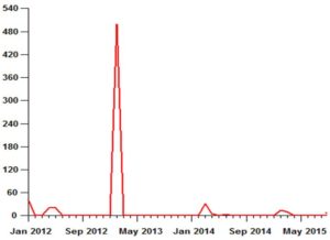
Figure 4 illustrates the problem that a successful promotion can accidentally create for inventory management. If such a spike arises from the natural, un-promoted demand, then the only way to maintain high fill rates is to provide safety stocks large enough to cope with these random surges. In this case, the big spike in demand of 500 units in February 2013 was the result of a one-time promotion.

Taking Account of Promotions to Improve Inventory Management

Unwittingly treating the spike in the example above as part of the natural demand variability results in a poor fill rate. To achieve a target service level of, say, 95% with a lead time of one month would require a reorder point of 38 units, computed as the sum of an expected forecast over the one month replenishment lead time of 21 units supplemented by a safety stock of 17 units. This investment would result in a disappointing fill rate of only 36%.

However, recognizing that the spike is a one-time promotion and replacing the 500 units with 0 obviously would make a big difference. The reorder point would drop from 38 units to 31 (the sum of an expected demand of 7 units and a safety stock of 24 units) and the fill rate would increase to 94%.

Of course, it is not ok to just throw out inconvenient demand spikes whenever they make life uncomfortable; there has to be a valid “business story” behind the adjustment of historical demand. If the spike is the result of a data processing error, then by all means, fix it. If the spike coincides with a promotion, then replacing the spike with, say, the median demand (often zero, as in this example) will result in a much more sustainable inventory investment that still meets aggressive performance targets. Future promotions of the same type on the same item will require some extra effort to prepare for the temporary surge in demand, but the recommended reorder point will be correct in the long run.

Thomas Willemain, PhD, co-founded Smart Software and currently serves as Senior Vice President for Research. Dr. Willemain also serves as Professor Emeritus of Industrial and Systems Engineering at Rensselear Polytechnic Institute and as a member of the research staff at the Center for Computing Sciences, Institute for Defense Analyses.

Improve Forecast Accuracy, Eliminate Excess Inventory, & Maximize Service Levels

In this Video Dr. Thomas Willemain, co–Founder and SVP Research, talks about forecast-based inventory management policy, also known as MRP logic. This is the fourth in our series on major approaches to managing inventory.  We begin by looking at some very simple and then more robust models of inventory dynamics that help us determine how much to order or manufacture and when. We then consider how to calculate lead time and account for lead time variability. Tom concludes by describing the importance of safety stock, it’s role in properly buffering against demand and supply uncertainty, and how best to calculate it. 

Anybody doing the job knows that managing inventory can be stressful. Common stressors include: Customers with “special” requests, IT departments with other priorities, balky ERP systems running on inaccurate data, raw material shortages, suppliers with long lead times in far-away countries where production often stops for various reasons and more. This note will address one particular and ever-present source of stress: demand variability.

Everybody Has a Forecasting Problem

Suppose you manage a large fleet of spare parts. These might be surgical equipment for your hospital, or repair parts for your power station. Your mission is to maximize up time. Your enemy is down time. But because breakdowns hit at random, you are constantly in reactive mode. You might hope for rescue from forecasting technologies. But forecasts are inevitably imperfect to some degree: the element of surprise is always present.  You might wait for Internet of Things (IOT) tech to be deployed on your equipment to monitor and detect impending failures, helping you schedule repairs well in advance. But you know you can’t meter up the thousands of small things that can fail and disable a big thing.

So, you decide to combine forecasting with inventory management and build buffers or safety stock to protect against surprise spikes in demand. Now you have to work out how much safety stock to maintain, knowing that too little means vulnerability and too much means bloat.

Suppose you handle finished goods inventories for a make-to-stock company. Your problem is essentially the same as in managing service parts: You have external customers and uncertain demand. But you may also have additional problems in terms of synchronizing multiple suppliers of components that you assemble into finished goods. The suppliers want you to tell them how much of their stuff to make so you can make your stuff, but you don’t know how much of your own stuff you’ll need to make.

Finally, suppose you handle finished goods in a build-to-order company. You might think that you no longer have a forecasting problem, since you don’t build until you are paid to build. But you do have a forecasting problem. Since your finished goods might be assembled from a mixture of components and sub-assemblies, you have to translate some forecast of finished goods demand to work out a forecast of those components. Otherwise, you will go to make your finished goods and discover that you don’t have a required component and have to wait until you can re-actively assemble everything you need. And your customers might not be willing to wait.

So, everybody has a forecasting problem.

What Makes Forecasting Difficult

Forecasting can be quick, easy and dead accurate – as long as the world is simple. If demand for your product is 10 units every week, month after month, you can make very accurate forecasts. But life is not quite like that. If you’re lucky and life is almost like that – maybe weekly demand is more like {10, 9, 10, 8, 12, 10, 10…} — you can still make very accurate forecast and just make minor adjustments around the edges. But if life is as it more often is – maybe weekly demand looks like {0, 0, 7, 0, 0, 0, 23, 0 …} – demand forecasting is difficult indeed. The key distinction is demand variability: it’s the zigging and zagging that creates the pain.

Safety Stock Takes Over Where Forecasting Leaves Off

Statistical forecasting methods are an important part of the solution. They let you squeeze as much advantage as possible from the historical patterns of demand your company has recorded for each item. The job of forecasts is to describe what is typical, which provides the base on which to cope with randomness in demand. Statistical forecasting techniques work by finding “big picture” features in demand records, such as trend and seasonality, then projecting those into the future. They all implicitly assume that whatever patterns exist now will persist, so 5% growth will continue, and July demand will always be 20% higher than February demand. To get to that point, statistical forecasting methods use some form of averaging to smother the “noise” in the demand history.

But then the rest of the job falls on inventory management, because the atypical, random component of future demand will still be a hassle in the future. This inevitable level of uncertainty has to be handled by the “shock-absorber” called safety stock.

The same methods that produce forecasts of trend and/or seasonality can be used to estimate the amount of forecast error. This has to be done carefully using a method called “holdout analysis”.  It works like this. Suppose you have 365 observations of daily demand for Item X, which has a replenishment lead time of 10 days. You want to know how many units will be demanded over some future 10-day period. You might input the first 305 days of demand history into the forecasting technique and get forecasts for the next 10 days, days 306-315.

The answer gives you one estimate of the 10-day total demand. Importantly, it also gives you one estimate of the variability around that forecast, i.e., the forecast error, the difference between what actually happened in days 306-315 and what was forecasted. Now you can repeat the process, this time using the first 306 days to forecast the next 10, the first 307 days to forecast the next 10, etc. You end up with 52 honest estimates of the variability of total demand over a 10-day lead time. Suppose 95% of those estimates are less than 28 units. Then 28 units would be a pretty safe safety stock to add to the forecast, since you will run into shortages only 5% of the time.

Modern statistical software does these calculations automatically. It can ease at least one of the chronic headaches of inventory management by helping you cope with demand variability.

This blog defines and compares the three most commonly used inventory control policies. It should be helpful both to those new to the field and also to experienced people contemplating a possible change in their company’s policy. The blog also considers how demand forecasting supports inventory management, choice of which policy to use, and calculation of the inputs that drive these policies. Think of it as an abbreviated piece of Inventory 101.

Scenario

You are managing a particular item. The item is important enough to your customers that you want to carry enough inventory to avoid stocking out. However, the item is also expensive enough that you also want to minimize the amount of cash tied up in inventory. The process of ordering replenishment stock is sufficiently expensive and cumbersome that you also want to minimize the number of purchase orders you must generate. Demand for the item is unpredictable.  So is the replenishment lead time between when you detect the need for more and when it arrives on the shelf ready for use or shipment. 

Your question is “How do I manage this item? How do I decide when to order more and how much to order?”  When making this decision there are different approaches you can use.  This blog outlines the most commonly used inventory planning policies:  Periodic Order Up To (T, S), Reorder Point/Order Quantity (R, Q), and Min/Max (s, S).  These approaches are often embedded in ERP systems and enable companies to generate automatic suggestions of what and when to order.  To make the right decision, you’ll need to know how each of these approaches are designed to work and the advantages and limitations of each approach.    

Periodic review, order-up-to policy

The shorthand notation for this policy is (T, S), where T is the fixed time between orders and S is the order-up-to-level.

When to order: Orders are placed like clockwork every T days. The used of a fixed reorder interval is helpful to firms that cannot keep track of their inventory level in real time or who prefer to issue orders to suppliers at scheduled intervals.

How much to order: The inventory level is measured and the gap computed between that level and the order-up-to level S. If the inventory level is 7 units and S = 10, then 3 units are ordered.

Comment: This is the simplest policy to implement but also the least agile in responding to fluctuations in demand and/or lead time. Also, note that, while the order size would be adequate to return the inventory level to S if replenishment were immediate, in practice there will be some replenishment delay during which time the inventory continues to drop, so the inventory level will rarely reach all the way up S.

Continuous review, fixed order quantity policy (Reorder Point, Order Quantity)

The shorthand notation for this policy is (R, Q), where R is the reorder point and Q is the fixed order quantity.

When to order: Orders are placed as soon as the inventory drops to or below the reorder point, R. In theory, the inventory level is checked constantly, but in practice it is usually checked periodically at the beginning or end of each workday. 

How much to order: The order size is always fixed at Q units.

Comment: (R, Q) is more responsive than (S, T) because it reacts more quickly to signs of imminent stockout. The value of the fixed order quantity Q may not be entirely up to you. Often suppliers can dictate terms that restrict your choice of Q to values compatible with minima and multiples. For example, a supplier may insist on an order minimum of 20 units and always be a multiple of 5. Thus orders sizes must be either 20, 25, 30, 35, etc. (This comment also applied to the two other inventory policies.)

Continuous review, order-up-to policy (Min/Max)

The shorthand notation for this policy is (s, S), sometimes called “little s, big S” where s is the reorder point and S is the order-up-to level. This policy is more commonly called (Min, Max).

When to order: Orders are placed as soon as the inventory drops to or below the Min. As with (R, Q), the inventory level is supposedly monitored constantly, but in practice it is usually checked at the end of each workday. 

How much to order: The order size varies. It equals the gap between the Max and the current inventory at the moment that the Min is reached or breached.

Comment: (Min, Max) is even more responsive than (R, Q) because it adjusts the order size to take account of how much the inventory has fallen below the Min. When demand is either zero or one units, a common variation sets Min = Max -1; this is called the “base stock policy.”

Another policy choice: What happens if I stock out?

As you can imagine, each policy is likely to lead to a different temporal sequence of inventory levels (see Figure 1 below). There is another factor that influences how events play out over time: the policy you select for dealing with stockouts. Broadly speaking, there are two main approaches.

Backorder policy: If you stock out, you keep track of the order and fill it later.  Under this policy, it is sensible to speak of negative inventory. The negative inventory represents the number of backorders that need to be filled. Presumably, any customer forced to wait gets first dibs when replenishment arrives. You are likely to have a backorder policy on items that are unique to your business that your customer cannot purchase elsewhere.

Loss policy: If you stock out, the customer turns to another source to fill their order. When replenishment arrives, some new customer will get those new units. Inventory can never go below zero.  Choose this policy for commodity items that can easily be purchased from a competitor.  If you don’t have it in stock, your customer will most certainly go elsewhere. 

The role of demand forecasting in inventory control

Choice of control parameters, such as the values of Min and Max, requires inputs from some sort of demand forecasting process.

Traditionally, this has meant determining the probability distribution of the number of units that will be demanded over a fixed time interval, either the lead time in (R, Q) and (Min, Max) systems or T + lead time in (T, S) systems. This distribution has been assumed to be Normal (the famous “bell-shaped curve”).  Traditional methods have been expanded where the demand distribution isn’t assumed to be normal but some other distribution (i.e. Poisson, negative binomial, etc.) 

These traditional methodologies have several deficiencies.

• First, it usually ignores the problem of undershoot, in which demand drops inventory not just to the reorder point but below it. Assuming no undershoot leads to overestimates of service levels and fill rates.

• Second, the probability distribution of demand is very often not even close to “bell-shaped” or whatever assumed distribution was selected –  especially for items with intermittent demand such as spares and service parts.

• Third, accurate estimates of inventory operating costs require analysis of the entire replenishment cycle (from one replenishment to the next), not merely the part of the cycle that begins with inventory hitting the reorder point.

• Finally, replenishment lead times are typically unpredictable or random, not fixed. Many models assume a fixed lead time based on an average, vendor quoted lead time, or average lead time + safety time.

Fortunately, better inventory planning and inventory optimization software exists based on generating a full range of random demand scenarios, together with random lead times. These scenarios “stress test” any proposed pair of inventory control parameters and assess their expected performance. Users can not only choose between policies (i.e. Min, Max vs. R, Q) but also determine which variation of the proposed policy is best (i.e. Min, Max of 10,20 vs. 15, 25, etc.) Examples of these scenarios are given below.

The process of ordering replenishment stock is sufficiently expensive and cumbersome that you also want to minimize the number of purchase orders you must generate

Choosing among inventory control policies

Which policy is right for you? There is a clear pecking order in terms of item availability, with (Min, Max) first, (R, Q) second, and (T, S) last. This order derives from the responsiveness of the policy to fluctuations in the randomness of demand and replenishment. The order reverses when considering ease of implementation.

How do you “score” the performance of an inventory policy? There are two opposing forces that must be balanced: cost and service.

Inventory cost can be expressed either as inventory investment or inventory operating cost. The former is the dollar value of the items waiting around to be used. The latter is the sum of three components: holding cost (the cost of the “care and feeding of stuff on the shelf”), ordering cost (basically the cost of cutting a purchase order and receiving that order), and shortage cost (the penalty you pay when you either lose a sale or force a customer to wait for what they want).

Service is usually measured by service level and fill rate.  Service level is the probability that an item requested is shipped immediately from stock. Fill rate is the proportion of units demanded that are shipped immediately from stock. As a former professor, I think of service level as an all-or-nothing grade: If a customer needs 10 units and you can provide only 9, that’s an F. Fill rate is a partial credit grade: 9 out of 10 is 90%.

When you decide on the values of inventory control policies, you are striking a balance between cost and service. You can provide perfect service by keeping an infinite inventory. You can hold costs to zero by keeping no inventory. You must find a sensible place to operate between these two ridiculous extremes. Generating and analyzing demand scenarios can quantify the consequences of your choices.

A demonstration of the differences between two inventory control policies

We now show how on-hand inventory evolves differently under two policies. The two policies are (R, Q) and (Min, Max) with backorders allowed. To keep the comparison fair, we set Min = R and Max = R+Q, use a fixed lead time of five days, and subject both policies to the same sequence of daily demands over 365 simulated days of operation.

Figure 1 shows daily on-hand inventory under the two policies subjected to the same pattern of daily demand. In this example, the (Min, Max) policy has only two periods of negative inventory during the year, while the (R, Q) policy has three. The (Min, Max) policy also operates with a smaller average number of units on hand. Different demand sequences will produce different results, but in general the (Min, Max) policy performs better.

Note that the plots of on-hand inventory contain information needed to compute both cost and availability metrics.

Figure 1: Comparison of daily on-hand inventory under two inventory policies

Role of Inventory Planning Software

Best of Breed Inventory Planning, Forecasting, and Optimization systems can help you determine which type of policy (is it better to use Min/Max over R,Q) and what sets of inputs are optimal (i.e. what should I enter for Min and Max).  Best of breed inventory planning and demand forecasting systems can help you develop these optimized inputs so that you can regularly populate and update your ERP systems with accurate replenishment drivers.

Summary

We defined and described the three most commonly used inventory control policies: (T, S), (R, Q) and (Min, Max), along with the two most common responses to stockouts: backorders or lost orders. We noted that these policies require successively greater effort to implement but also have successively better average performance. We highlighted the role of demand forecasts in assessing inventory control policies. Finally, we illustrated how choice of policy influences the day-to-day level of on-hand inventory.

Summary

Setting a target service level or fill rate is a strategic decision about inventory risk management. Choosing service levels can be difficult. Relevant factors include current service levels, replenishment lead times, cost constraints, the pain inflicted by shortages on you and your customers, and your competitive position. Target setting is often best approached as a collaboration among operations, sales and finance. Inventory optimization software is an essential tool in the process.

Service Level Choices

Service level is the probability that no shortages occur between when you order more stock and when it arrives on the shelf. The reasonable range of service levels is from about 70% to 99%. Levels below 70% may signal that you don’t care about or can’t handle your customers. Levels of 100% are almost never appropriate and usually indicate a hugely bloated inventory.

Factors Influencing Choice of Service Level

Several factors influence the choice of service level for an inventory item. Here are some of the more important.

Current service levels:
A reasonable place to start is to find out what your current service levels are for each item and overall. If you are already in good shape, then the job becomes the easier one of tweaking an already-good solution. If you are in bad shape now, then setting service levels can be more difficult. Surprisingly few companies have data on this important metric across their whole fleet of inventory items. What often happens is that reorder points grow willy-nilly from choices made in corporate pre-history and are rarely, sometimes never, systematically reviewed and updated. Since reorder points are a major determinant of service levels, it follows that service levels “just happen”. Inventory optimization software can convert your current reorder points and lead times into solid estimates of your current service levels. This analysis often reveals subset of items with service levels either too high or too low, in which case you have guidance about which items to adjust down or up, respectively.

Replenishment lead times:
Some companies adjust service levels to match replenishment lead times. If it takes a long time to make or buy an item, then it takes a long time to recover from a shortage. Accordingly, they bump up service levels on long-lead-time items and reduce them on items for which backlogs will be brief.

Cost constraints:
Inventory optimization software can find the lowest-cost ways to hit high service level targets, but aggressive targets inevitably imply higher costs. You may find that costs constrain your choice of service level targets. Costs come in various flavors. “Inventory investment” is the dollar value of inventory. “Operating costs” include both holding costs and ordering costs. Constraints on inventory investment are often imposed on inventory executives and always imply ceilings on service level targets; software can make these relationships explicit but not take away the necessity of choice. It is less common to hear of ceilings on operating costs, but they are always at least a secondary factor arguing for lower service levels.

Shortage costs:
Shortage costs depend on whether your shortage policy calls for backorders or lost sales. In either case, shortage costs work counter to inventory investment and operating costs by arguing for higher service levels. These costs may not always be expressed in dollar terms, as in the case of medical/surgical supplies, where shortage costs are denominated in morbidity and mortality.

Competition:
The closer your company is to dominating its market, the more you can ease back on service levels to save money. However, easing back too far carries risks: It encourages potential customers to look elsewhere, and it encourages competitors. Conversely, high product availability can go far to bolstering the position of a minor player.

Collaborative Targeting

Inventory executives may be the ones tasked with setting service level targets, but it may be best to collaborate with other functions when making these calls. Finance can share any “red lines” early in the process, and they should be tasked with estimating holding and ordering costs. Sales can help with estimating shortage costs by explaining likely customer reactions to backlogs or lost sales.

The Role of Inventory Optimization and Planning Software

Without inventory optimization software, setting service level targets is pure guesswork: It is impossible to know how any given target will play out in terms of inventory investment, operating costs, shortage costs. The software can compute the detailed, quantitative tradeoff curves required to make informed choices or even recommend the target service level that results in the lowest overall cost considering holding costs, ordering costs, and stock out costs. However, not all software solutions are created equal. You might enter a user defined 99% service level into your inventory planning system or the system could recommend a target service – but it doesn’t mean you will actually hit that stated service level. In fact, you might not even come close to hitting it and achieve a much lower service level. We’ve observed situations where a targeted service level of 99% actually achieved a service level of just 82%! Any decisions made as a result of the target will result in unintended misallocation of inventory, very costly consequences, and lots of explaining to do.So be sure to check out our blog article on how to measure the accuracy of your service level forecast so you don’t make this costly mistake.