For some of our customers, weather has a significant influence on demand. Extreme short-term weather events like fires, droughts, hot spells, and so forth can have a significant near-term influence on demand.

There are two ways to factor weather into a demand forecast: indirectly and directly. The indirect route is easier using the scenario-based approach of Smart Demand Planner. The direct approach requires a tailored special project requiring additional data and hand-crafted modeling.

Indirect Accounting for Weather

The standard model built into Smart Demand Planner (SDP) accommodates weather effects in four ways:

1. If the world is steadily getting warmer/colder/drier/wetter in ways that impact your sales, SDP detects these trends automatically and incorporates them into the demand scenarios it generates.
2. If your business has a regular rhythm in which certain days of the week or certain months of the year have consistently higher or lower-than-average demand, SDP also automatically detects this seasonality and incorporates it into its demand scenarios.
3. Often it is the cussed randomness of weather that interferes with forecast accuracy. We often refer to this effect as “noise”. Noise is a catch-all term that incorporates all kinds of random trouble. Besides weather, a geopolitical flareup, the surprise failure of a regional bank, or a ship getting stuck in the Suez Canal can and have added surprises to product demand. SDP assesses the volatility of demand and reproduces it in its demand scenarios.
4. Management overrides. Most of the time, customers let SDP churn away to automatically generate tens of thousands of demand scenarios. But if users feel the need to touch up specific forecasts using their insider knowledge, SDP can make that happen through management overrides.

Direct Accounting for Weather

Sometimes a user will be able to articulate subject matter expertise linking factors outside their company (such as interest rates or raw materials costs or technology trends) to their own aggregate sales. In these situations, Smart Software can arrange for one-off special projects that provide alternative (“causal”) models to supplement our standard statistical forecasting models. Contact your Smart Software representative to discuss a possible causal modeling project.

Meanwhile, don’t forget your umbrella.

​When you should use traditional extrapolative forecasting techniques.

With so much hype around new Machine Learning (ML) and probabilistic forecasting methods, the traditional “extrapolative” or “time series” statistical forecasting methods seem to be getting the cold shoulder.  However, it is worth remembering that these traditional techniques (such as single and double exponential smoothing, linear and simple moving averaging, and Winters models for seasonal items) often work quite well for higher volume data. Every method is good for what it was designed to do.  Just apply each appropriately, as in don’t bring a knife to a gunfight and don’t use a jackhammer when a simple hand hammer will do. 

Extrapolative methods perform well when demand has high volume and is not too granular (i.e., demand is bucketed monthly or quarterly). They are also very fast and do not use as many computing resources as probabilistic and ML methods. This makes them very accessible.

Are the traditional methods as accurate as newer forecasting methods?  Smart has found that extrapolative methods do very poorly when demand is intermittent. However, when demand is higher volume, they only do slightly worse than our new probabilistic methods when demand is bucketed monthly.  Given their accessibility, speed, and the fact you are going to apply forecast overrides based on business knowledge, the baseline accuracy difference here will not be material.

The advantage of more advanced models like Smart’s GEN2 probabilistic methods is when you need to predict patterns using more granular buckets like daily (or even weekly) data.  This is because probabilistic models can simulate day of the week, week of the month, and month of the year patterns that are going to be lost with simpler techniques.  Have you ever tried to predict daily seasonality with a Winter’s model? Here is a hint: It’s not going to work and requires lots of engineering.

Probabilistic methods also provide value beyond the baseline forecast because they generate scenarios to use in stress-testing inventory control models. This makes them more appropriate for assessing, say, how a change in reorder point will impact stockout probabilities, fill rates, and other KPIs. By simulating thousands of possible demands over many lead times (which are themselves presented in scenario form), you’ll have a much better idea of how your current and proposed stocking policies will perform. You can make better decisions on where to make targeted stock increases and decreases.

So, don’t throw out the old for the new just yet. Just know when you need a hammer and when you need a jackhammer.

Probabilistic scenarios are sequences of data points generated to represent potential real-world situations. Unlike scenarios in war games or other simulations, these are synthetic time series used as inputs to system models or as intuition-builders for decision-makers.

For instance, scenarios of future item demand can be fed into Monte Carlo simulation models of inventory control systems, thereby creating a virtual laboratory in which to explore the consequences of management decisions, such as changing reorder points and/or order quantities. In addition, plots of metrics like on-hand inventory or stockouts can help inventory planners deepen their “feel” for the randomness inherent in their operations.

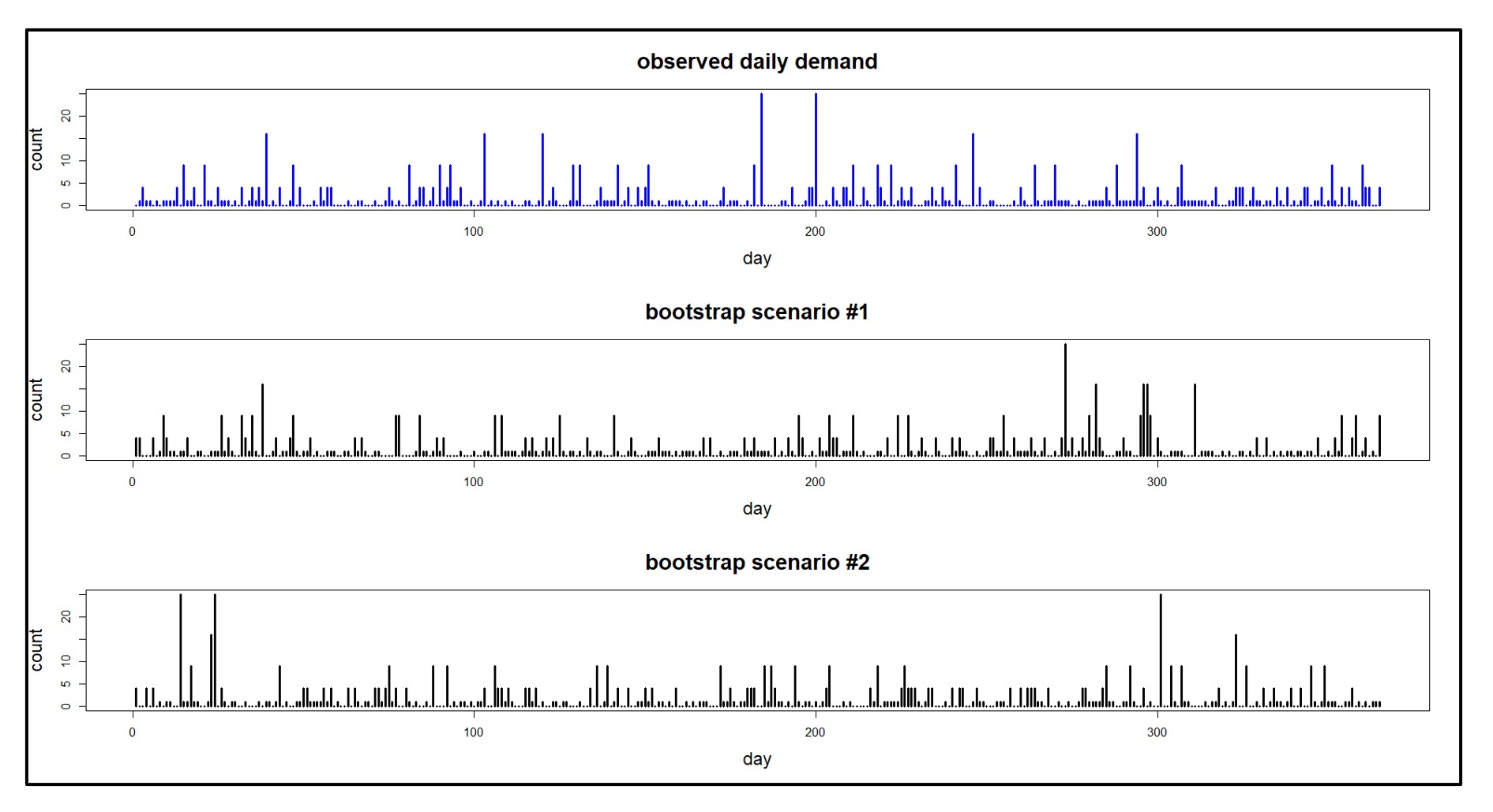
Figure 1 shows daily demand scenarios generated from a single observed demand series recorded over one year. Note that the same data generating process can “look quite different” in detail from sample to sample. This mimics real life.

Figure 1: An observed demand sequence and demand scenarios derived from it.

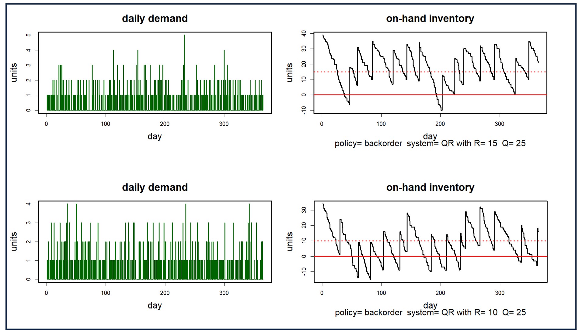
Figure 2 shows two demand scenarios and their consequences for stock on hand in a particular inventory control system. The difference between the two inventory plots illustrates the degree to which randomness in demand dominates the problem. The top plot shows two episodes of stockout, while the bottom plot shows nine. Averaging over many scenarios will clarify the typical values of Key Performance Metrics (KPIs) such as the average number of stockouts associated with any choice of Reorder Point and Order Quantity (which are 10 and 25, respectively, in Figure 2.)

Figure 2: Two demand scenarios and their consequences for on-hand inventory

In this note, we’ll describe techniques for creating scenarios and list criteria for evaluating scenario generators.

Criteria for Scenarios

As we’ll see below, there are several ways to create scenarios. No matter the source, what criteria define a “good” scenario? There are four main criteria: fidelity, variety, quantity, and cost. Fidelity summarizes how accurately a scenario imitates real-world situations. High fidelity means the scenarios mirror actual events closely, providing a solid foundation for analysis and decision-making. Variety describes the diversity of scenarios a generator can create. A versatile generator can simulate a wide range of potential situations, allowing for a thorough exploration of possibilities and risks. Quantity refers to how many scenarios a generator can produce. A generator that can create a large number of scenarios provides ample data for analysis. Cost considers both the computational and human resources required to produce the scenarios. An efficient scenario generator balances quality with resource usage, ensuring the effort is justified by the value and accuracy of the outcomes.

Scenario Generation

Again, think of a scenario as a time series. How are scenarios created?

1. Geppetto’s Workshop: This approach involves hand-crafting scenarios manually by experts. While it can yield high fidelity (realism), it is very resource-intensive and cannot easily generate variety, which requires a large number of scenarios.
2. Groundhog Day: This method involves repeatedly using a single real-world situation as input. While it’s realistic by definition and cost-effective (no resources are used beyond recording the data), this approach lacks variety and so cannot accurately reflect the diversity of real-world scenarios.
3. Parametric Models: Examples of parametric models are the classics studied in Statistics 101 classes: the Normal, exponential, Poisson, etc. The demand plots in Figure 2 are generated parametrically, being the squares of Poisson random variables. These models generate an unlimited number of low cost scenarios having good variety, but they may not always capture the complexity of real-world data, potentially compromising fidelity. When reality is more complicated, these models generate over-simplified scenarios.
4. Non-Parametric Time Series Bootstraps: This approach can score well on all criteria: fidelity, variety, quantity, and cost. It’s a versatile method that excels in creating massive numbers of realistic scenarios. The synthetic demand histories in Figure 1 are simple bootstrap samples based on the observed values in the top graph. (For some nitty-gritty details about generating scenarios, see the links below.)

Exploiting Scenarios

Scenarios prove their worth in two ways: As inputs to decision making and as intuition-builders. For instance, when demand scenarios are used as inputs to simulation models, they enable stress testing and performance estimation for system design. Scenarios can also serve as intuition-builders for decision-makers or system operators. Their visual representation aids in developing insight into and appreciation for the risks involved in making operational decisions, be they for demand forecasting or inventory management.

Scenario-based analysis is very computer intensive, especially when the scenarios are generated by bootstrapping. At Smart Software, computation happens in the cloud. Imagine the computational load involved in determining reorder points and order quantities for each of tens of thousands of inventory items using hundreds or thousands of demand simulations for each item. Further imagine the software not only evaluating a specific proposed reorder point/order quantity pair but roaming over the entire “design space” of pairs to find the best pair of control parameters for each item. To make this practical, we take advantage of the parallel processing power of the cloud. Essentially, each inventory item is assigned its own computer to use in the calculations, so that all that computing can happen simultaneously rather than sequentially. Now we can cut loose and really get you the results you need.

Learning More

Those interested in further technical details and references can find more information here.

What Makes a Probabilistic Forecast?

Probabilistic Forecasting for Intermittent Demand

People new to the jobs of “demand planner” or “supply planner” are likely to have questions about the various forecasting terms and methods used in their jobs. This note may help by explaining these terms and showing how they relate.

Demand Planning

Demand planning is about how much of what you have to sell will go out the door in the future, e.g., how many what-nots you will sell next quarter. Here are six methodologies often used in demand planning.

• Statistical Forecasting
  • These methods use demand history to forecast future values. The two most common methods are curve fitting and data smoothing.
  • Curve fitting matches a simple mathematical function, like the equation for a straight line (y= a +b∙t) or an interest-rate type curve (y=a∙b^t), to the demand history. Then it extends that line or curve forward in time as the forecast.
  • In contrast, data smoothing does not result in an equation. Instead it sweeps through the demand history, averaging values along the way, to create a smoother version of the history. These methods are called exponential smoothing and moving average. In the simplest case (i.e., in the absence of trend or seasonality, for which variants exist), the goal is to estimate the current average level of demand and use that as the forecast.
  • These methods produce “point forecasts”, which are single-number estimates for each future time period (e.g., “Sales in March will be 218 units”). Sometimes they come with estimates of potential forecast error bolted on using separate models of demand variability (“Sales in March will be 218 ± 120 units”).

• Probabilistic Forecasting
  • This approach keys on the randomness of demand and works hard to estimate forecast uncertainty. It regards forecasting less as an exercise in cranking out specific numbers and more as an exercise in risk management.
  • It explicitly models the variability in demand and uses that to present results in the form of large numbers of scenarios constructed to show the full range of possible demand sequences. These are especially useful in tactical supply planning tasks, such as setting reorder points and order quantities.

• Causal Forecasting
  • Statistical forecasting models use as inputs only the past demand history of the item in question. They regard the up-and-down wiggles in the demand plot as the end result of myriad unnamed factors (interest rates, the price of tea in China, phases of the moon, whatever). Causal forecasting explicitly identifies one or more influences (interest rates, advertising spend, competitors’ prices, …) that could plausibly influence sales. Then it builds an equation relating the numerical values of these “drivers” or “causal factors” to item sales. The equation’s coefficients are estimated by “regression analysis”.

• Judgemental Forecasting
  • Golden Gut. Despite the general availability of gobs of data, some companies pay little attention to the numbers and give greater weight to the subjective judgements of an executive deemed to have a “Golden Gut”, which allows him or her to use “gut feel” to predict what future demand will be. If that person has great experience, has spent a career actually looking at the numbers, and is not prone to wishful thinking or other forms of cognitive bias, the Golden Gut can be a cheap, fast way to plan. But there is good evidence from studies of companies run this way that relying on the Golden Gut is risky.
  • Group Consensus. More common is a process that uses a periodic meeting to create a group consensus forecast. The group will have access to shared objective data and forecasts, but members will also have knowledge of factors that may not be measured well or at all, such as consumer sentiment or the stories relayed by sales reps. It is helpful to have a shared, objective starting point for these discussions consisting of some sort of objective statistical analysis. Then the group can consider adjusting the statistical forecast. This process anchors the forecast in objective reality but exploits all the other information available outside the forecasting database.
  • Scenario Generation. Sometimes several people will meet and discuss “strategic what-if” questions. “What if we lose our Australian customers?” “What if our new product roll-out is delayed by six months?” “What if our sales manager for the mid-west jumps to a competitor?” These bigger-picture questions can have implications for item-specific forecasts and might be added to any group-consensus forecasting meeting.

• New product forecasting
  • New products, by definition, have no sales history to support statistical, probability, or causal forecasting. Subjective forecasting methods can always be used here, but these often rely on a dangerous ratio of hopes to facts. Fortunately, there is at least partial support for objective forecasting in the form of curve fitting.
  • A graph of the cumulative sales of an item often describes some sort of “S-curve”, i.e., a graph that starts at zero, builds up, then levels off to a final lifetime total sales. The curve gets its name because it looks like a letter S somehow smeared and stretched to the right. Now there are an infinite number of S-curves, so forecasters typically pick an equation and subjectively specify some key parameter values, like when sales will hit 25%, 50% and 75% of total lifetime sales and what that final level will be. This is also overtly subjective, but it produces detailed period-by-period forecasts that can be updated as experience builds up. Finally, S-curves are sometimes shaped to match the known history of a similar, predecessor product (“Sales for our last gizmo looked like this, so let’s use that as a template.”).

Supply Planning

Demand planning feeds into supply planning by predicting future sales (e.g., for finished goods) or usage (e.g., for spare parts). Then it is up to supply planning to make sure the items in question will be available to sell or to use.

• Dependent demand
  • Dependent demand is demand that can be determined by its relationship to demand for another item. For instance, a bill of materials may show that a little red wagon consists of a body, a pull bar, four wheels, two axles, and various fasteners to keep the wheels on the axles and connect the pull bar to the body. So if you hope to sell 10 little red wagons, you’d better make 10, which means you need 10×2 = 20 axles, 10×4 = 40 wheels, etc. Dependent demand governs raw materials purchasing, component and subsystems purchasing, even personnel hiring (10 wagons need one high-school kid to put them together over a 1 hour shift).
  • If you have multiple products with partially overlapping bills of materials, you have a choice of two forecasting approaches. Suppose you sell not only little red wagons but little blue baby carriages and that both use the same axles. To predict the number of axles you need you could (1) predict the dependent demand for axles from each product and add the forecasts or (2) observe the total demand history for axles as its own time series and forecast that separately. Which works better is an empirical question that can be tested.

• Inventory management
  • Inventory management entails many different tasks. These include setting inventory control parameters such as reorder points and order quantities, reacting to contingencies such as stockouts and order expediting, setting staffing levels, and selecting suppliers.

• Forecasting plays a role in the first three. The number of replenishment orders that will be made in a year for each product determines how many people are needed to cut PO’s. The number and severity of stockouts in a year determines the number of contingencies that must be handled. The number of PO’s and stockouts in a year will be random but be governed by the choices of inventory control parameters. The implications of any such choices can be modeled by inventory simulations. These simulations will be driven by detailed demand scenarios generated by probabilistic forecasts.

​

Every field, including forecasting, accumulates folk wisdom that eventually starts masquerading as “best practices.”  These best practices are often wise, at least in part, but they often lack context and may not be appropriate for certain customers, industries, or business situations.  There is often a catch, a “Yes, but”. This note is about six usually true forecasting precepts that nevertheless do have their caveats.

1. Organize your company around a one-number forecast. This sounds sensible: it’s good to have a shared vision. But each part of the company will have its own idea about which number is the number. Finance may want quarterly revenue, Marketing may want web site visits, Sales may want churn, Maintenance may want mean time to failure. For that matter, each unit probably has a handful of key metrics. You don’t need a slogan – you need to get your job done.

2. Incorporate business knowledge into a collaborative forecasting process. This is a good general rule, but if your collaborative process is flawed, messing with a statistical forecast via management overrides can decrease accuracy. You don’t need a slogan – you need to measure and compare the accuracy of any and all methods and go with the winners.

3. Forecast using causal modeling. Extrapolative forecasting methods take no account of the underlying forces driving your sales, they just work with the results. Causal modeling takes you deeper into the fundamental drivers and can improve both accuracy and insight. However, causal models (implemented through regression analysis) can be less accurate, especially when they require forecasts of the drivers (“predictions of the predictors”) rather than simply plugging in recorded values of lagged predictor variables. You don’t need a slogan: You need a head-to-head comparison.

4. Forecast demand instead of shipments. Demand is what you really want, but “composing a demand signal” can be tricky: what do you do with internal transfers? One-off’s?  Lost sales? Furthermore, demand data can be manipulated.  For example, if customers intentionally don’t place orders or try to game their orders by ordering too far in advance, then order history won’t be better than shipment history.  At least with shipment history, it’s accurate:  You know what you shipped. Forecasts of shipments are not forecasts of  “demand”, but they are a solid starting point.

5. Use Machine Learning methods. First, “Machine learning” is an elastic concept that includes an ever-growing set of alternatives. Under the hood of many ML advertised models is just an auto-pick an extrapolative forecast method (i.e., best fit) which while great at forecasting normal demand, has been around since the 1980’s (Smart Software was the first company to release an auto-pick method for the PC).   ML models are data hogs that require larger data sets than you may have available. Properly choosing then training an ML model requires a level of statistical expertise that is uncommon in many manufacturing and distribution businesses. You might want to find somebody to hold your hand before you start playing this game.

6. Removing outliers creates better forecasts. While it is true that very unusual spikes or drops in demand will mask underlying demand patterns such as trend or seasonality, it isn’t always true that you should remove the spikes. Often these demand surges reflect the uncertainty that can randomly interfere with your business and thus need to be accounted for.  Removing this type of data from your demand forecast model might make the data more predictable on paper but will leave you surprised when it happens again. So, be careful about removing outliers, especially en masse.