
In my previous post in this series on essential concepts, “What is ‘A Good Forecast’”, I discussed the basic effort to discover the most likely future in a demand planning scenario. I defined a good forecast as one that is unbiased and as accurate as possible. But I also cautioned that, depending on the stability or volatility of the data we have to work with, there may still be some inaccuracy in even a good forecast. The key is to have an understanding of how much.
This topic, managing uncertainty, is the subject of post by my colleague Tom Willemain, “The Average is not the Answer”. His post lays out the theory for responsibly confronting the limits of our predictive ability. It’s important to understand how this actually works.
As I briefly touched on at the end of my previous post, our approach begins with something called a “sliding simulation”. We estimate how accurately we are predicting the future by using our forecasting techniques on an older portion of history, excluding the most recent data. We can then compare what we would have predicted for the recent past with our actual real world information about what happened. This is a reliable method to estimate how closely we are predicting future demand.
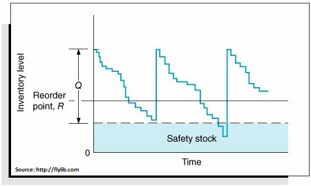
Safety stock, a carefully measured buffer in inventory level we stock above our prediction of most likely demand, is derived from the estimate of forecast error coming out of the “sliding simulation”. This approach to dealing with the accuracy of our forecasts efficiently balances between ignoring the threat of the unpredictable and costly overcompensation.
 In more technical detail: the forecasts errors that are estimated by this sliding simulation process indicate the level of uncertainty. We use these errors to estimate the standard deviation of the forecasts. Now, with regular demand, we can assume the forecasts (which are estimates of future behavior) are best represented by a bell-shaped probability distribution—what statisticians call the “normal distribution”. The center of that distribution is our point forecast. The width of that distribution is the standard deviation of the “sliding simulation” forecast from the known actual values—we obtain this directly from our forecast error estimates.
Once we know the specific bell shaped curve associated with the forecast, we can easily estimate the safety stock buffer that is needed. The only input from us is the “service level” that is desired, and the safety stock at that service level can be ascertained. (The service level is essentially a measure of how confident we need to be in our inventory stocking levels, with increasing confidence requiring corresponding expenditures on extra inventory.) Notice, we are assuming that the correct distribution to use is the normal distribution. This is correct for most demand series where you have regular demand per period. It fails when demand is sporadic or intermittent.
In the next piece in this series, I’ll discuss how Smart Forecasts deals with estimating safety stock in those cases of intermittent demand, when the assumption of normality is incorrect.
Nelson Hartunian, PhD, co-founded Smart Software, formerly served as President, and currently oversees it as Chairman of the Board. He has, at various times, headed software development, sales and customer service.

Related Posts

Forecast-Based Inventory Management for Better Planning
Forecast-based inventory management, or MRP (Material Requirements Planning) logic, is a forward-planning method that helps businesses meet demand without overstocking or understocking. By anticipating demand and adjusting inventory levels, it maintains a balance between meeting customer needs and minimizing excess inventory costs. This approach optimizes operations, reduces waste, and enhances customer satisfaction.

Leveraging Epicor Kinetic Planning BOMs with Smart IP&O to Forecast Accurately
In this blog, we explore how leveraging Epicor Kinetic Planning BOMs with Smart IP&O can transform your approach to forecasting in a highly configurable manufacturing environment. Discover how Smart, a cutting-edge AI-driven demand planning and inventory optimization solution, can simplify the complexities of predicting finished goods demand, especially when dealing with interchangeable components. Learn how Planning BOMs and advanced forecasting techniques enable businesses to anticipate customer needs more accurately, ensuring operational efficiency and staying ahead in a competitive market.

Daily Demand Scenarios
In this Videoblog, we will explain how time series forecasting has emerged as a pivotal tool, particularly at the daily level, which Smart Software has been pioneering since its inception over forty years ago. The evolution of business practices from annual to more refined temporal increments like monthly and now daily data analysis illustrates a significant shift in operational strategies.
Recent Posts
 Forecast-Based Inventory Management for Better PlanningForecast-based inventory management, or MRP (Material Requirements Planning) logic, is a forward-planning method that helps businesses meet demand without overstocking or understocking. By anticipating demand and adjusting inventory levels, it maintains a balance between meeting customer needs and minimizing excess inventory costs. This approach optimizes operations, reduces waste, and enhances customer satisfaction. […]
 Make AI-Driven Inventory Optimization an Ally for Your OrganizationIn this blog, we will explore how organizations can achieve exceptional efficiency and accuracy with AI-driven inventory optimization. Traditional inventory management methods often fall short due to their reactive nature and reliance on manual processes. Maintaining optimal inventory levels is fundamental for meeting customer demand while minimizing costs. The introduction of AI-driven inventory optimization can significantly reduce the burden of manual processes, providing relief to supply chain managers from tedious tasks. […]
 The Importance of Clear Service Level Definitions in Inventory ManagementInventory optimization software that supports what-if analysis will expose the tradeoff of stockouts vs. excess costs of varying service level targets. But first it is important to identify how “service levels” is interpreted, measured, and reported. This will avoid miscommunication and the false sense of security that can develop when less stringent definitions are used. Clearly defining how service level is calculated puts all stakeholders on the same page. This facilitates better decision-making. […]
 Future-Proofing Utilities: Advanced Analytics for Supply Chain OptimizationUtilities in the electrical, natural gas, urban water, and telecommunications fields are all asset-intensive and reliant on physical infrastructure that must be properly maintained, updated, and upgraded over time. Maximizing asset uptime and the reliability of physical infrastructure demands effective inventory management, spare parts forecasting, and supplier management. A utility that executes these processes effectively will outperform its peers, provide better returns for its investors and higher service levels for its customers, while reducing its environmental impact. […]
 The Cost of Spreadsheet PlanningCompanies that depend on spreadsheets for demand planning, forecasting, and inventory management are often constrained by the spreadsheet’s inherent limitations. This post examines the drawbacks of traditional inventory management approaches caused by spreadsheets and their associated costs, contrasting these with the significant benefits gained from embracing state-of-the-art planning technologies. […]

Inventory Optimization for Manufacturers, Distributors, and MRO
- Future-Proofing Utilities: Advanced Analytics for Supply Chain OptimizationUtilities in the electrical, natural gas, urban water, and telecommunications fields are all asset-intensive and reliant on physical infrastructure that must be properly maintained, updated, and upgraded over time. Maximizing asset uptime and the reliability of physical infrastructure demands effective inventory management, spare parts forecasting, and supplier management. A utility that executes these processes effectively will outperform its peers, provide better returns for its investors and higher service levels for its customers, while reducing its environmental impact. […]
 Centering Act: Spare Parts Timing, Pricing, and ReliabilityIn this article, we'll walk you through the process of crafting a spare parts inventory plan that prioritizes availability metrics such as service levels and fill rates while ensuring cost efficiency. We'll focus on an approach to inventory planning called Service Level-Driven Inventory Optimization. Next, we'll discuss how to determine what parts you should include in your inventory and those that might not be necessary. Lastly, we'll explore ways to enhance your service-level-driven inventory plan consistently. […]
 Why MRO Businesses Need Add-on Service Parts Planning & Inventory SoftwareMRO organizations exist in a wide range of industries, including public transit, electrical utilities, wastewater, hydro power, aviation, and mining. To get their work done, MRO professionals use Enterprise Asset Management (EAM) and Enterprise Resource Planning (ERP) systems. These systems are designed to do a lot of jobs. Given their features, cost, and extensive implementation requirements, there is an assumption that EAM and ERP systems can do it all. In this post, we summarize the need for add-on software that addresses specialized analytics for inventory optimization, forecasting, and service parts planning. […]
 5 Steps to Improve the Financial Impact of Spare Parts PlanningIn today’s competitive business landscape, companies are constantly seeking ways to improve their operational efficiency and drive increased revenue. Optimizing service parts management is an often-overlooked aspect that can have a significant financial impact. Companies can improve overall efficiency and generate significant financial returns by effectively managing spare parts inventory. This article will explore the economic implications of optimized service parts management and how investing in Inventory Optimization and Demand Planning Software can provide a competitive advantage. […]