In this article, we will review the “suggested orders” functionality in Epicor BisTrack, explain its limitations, and summarize how Smart Inventory Planning & Optimization (Smart IP&O) can help reduce inventory & minimize stock-outs by accurately assessing the tradeoffs between stockout risks and inventory costs.

Automating Replenishment in Epicor BisTrack
Epicor BisTrack’s “Suggested Ordering” can manage replenishment by suggesting what to order and when via reorder point-based policies such as min-max and/or manually specified weeks of supply. BisTrack contains some basic functionality to compute these parameters based on average usage or sales, supplier lead time, and/or user-defined seasonal adjustments. Alternatively, reorder points can be specified completely manually. BisTrack will then present the user with a list of suggested orders by reconciling incoming supply, current on hand, outgoing demand, and stocking policies.

How Epicor BisTrack “Suggested Ordering” Works
To get a list of suggested orders, users specify the methods behind the suggestions, including locations for which to place orders and how to determine the inventory policies that govern when a suggestion is made and in what quantity.

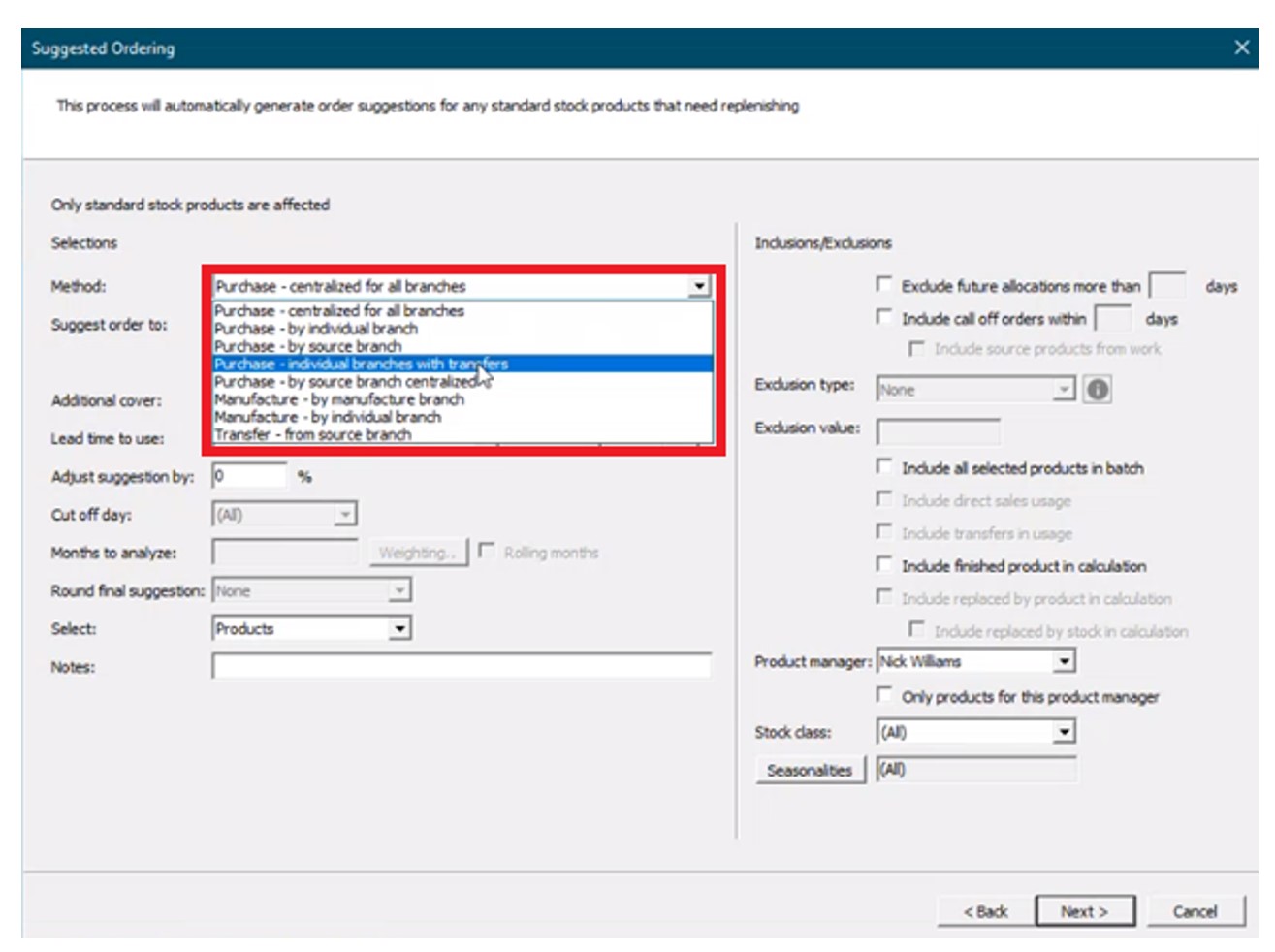
First, the “method” field is specified from the following options to determine what kind of suggestion is generated and for which location(s):

Purchase – Generate purchase order recommendations.

1. Centralized for all branches – Generates suggestions for a single location that buys for all other locations.
2. By individual branch – Generates suggestions for multiple locations (vendors would ship directly to each branch).
3. By source branch – Generates suggestions for a source branch that will transfer material to branches that it services (“hub and spoke”).
4. Individual branches with transfers – Generates suggestions for an individual branch that will transfer material to branches that it services (“hub and spoke”, where the “hub” does not need to be a source branch).

Manufacture – Generate work order suggestions for manufactured goods.

1. By manufacture branch.
2. By individual branch.

Transfer from source branch – Generate transfer suggestions from a given branch to other branches.

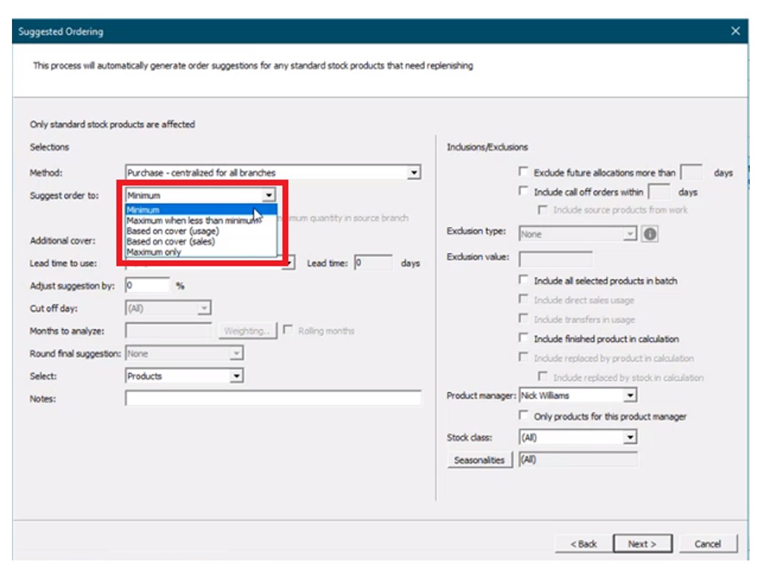
Next, the “suggest order to” is specified from the following options:

1. Minimum – Suggests orders “up to” the minimum on hand quantity (“min”). For any item where supply is less than the min, BisTrack will suggest an order suggestion to replenish up to this quantity.
2. Maximum when less than min – Suggests orders “up to” a maximum on-hand quantity when the minimum on-hand quantity is breached (e.g. a min-max inventory policy).

3. Based on cover (usage) – Suggests orders based on coverage for a user-defined number of weeks of supply with respect to a specified lead time. Given internal usage as demand, BisTrack will recommend orders where supply is less than the desired coverage to cover the difference.

4. Based on over (sales) – Suggests orders based on coverage for a user-defined number of weeks of supply with respect to a specified lead time. Given sales orders as demand, BisTrack will recommend orders where supply is less than the desired coverage to cover the difference.

5. Maximum only – Suggests orders “up to” a maximum on-hand quantity where supply is less than this max.

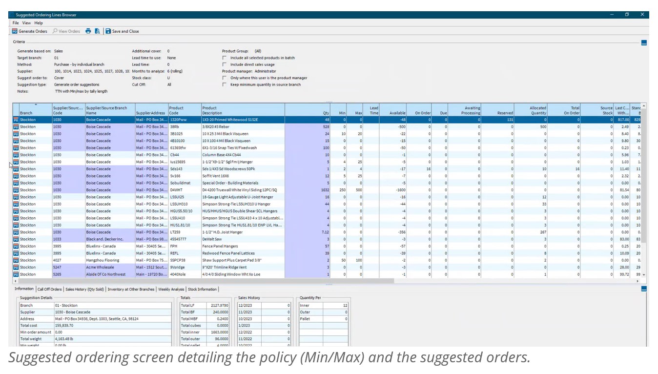
Finally, if allowing BisTrack to determine the reorder thresholds, users can specify additional inventory coverage as buffer stock, lead times, how many months of historical demand to consider, and can also manually define period-by-period weighting schemes to approximate seasonality. The user will be handed a list of suggested orders based on the defined criteria. A buyer can then generate POs for suppliers with the click of a button.

Limitations

Rule-of-thumb Methods

While BisTrack enables organizations to generate reorder points automatically, these methods rely on simple averages that do not capture seasonality, trends, or the volatility in an item’s demand. Averages will always lag behind these patterns and are unable to pick up on trends. Consider a highly seasonal product like a snow shovel—if we take an average of Summer/Fall demand as we approach the Winter season instead of looking ahead, then the recommendations will be based on the slower periods instead of anticipating upcoming demand. Even if we consider an entire years’ worth of history or more, the recommendations will overcompensate during the slower months and underestimate the busy season without manual intervention.

Rule of thumb methods also fail when used to buffer against supply and demand variability.  For example, the average demand over the lead time might be 20 units.  However, a planner would often want to stock more than 20 units to avoid stocking out if lead times are longer than expected or demand is higher than the average.  BisTrack allows users to specify the reorder points based on multiples of the averages.  However, because the multiples don’t account for the level of predictability and variability in the demand, you’ll always overstock predictable items and understock unpredictable ones.   Read this article to learn more about why multiples of the average fail when it comes to developing the right reorder point.

Manual Entry
Speaking of seasonality referenced earlier, BisTrack does allow the user to approximate it through the use of manually entered “weights” for each period. This forces the user to have to decide what that seasonal pattern looks like—for every item. Even beyond that, the user must dictate how many extra weeks of supply to carry to buffer against stockouts, and must specify what lead time to plan around. Is 2 weeks extra supply enough? Is 3 enough? Or is that too much? There is no way to know without guessing, and what makes sense for one item might not be the right approach for all items.

Intermittent Demand
Many BisTrack customers may consider certain items “unforecastable” because of the intermittent or “lumpy” nature of their demand. In other words, items that are characterized by sporadic demand, large spikes in demand, and periods of little or no demand at all. Traditional methods—and rule-of-thumb approaches especially—won’t work for these kinds of items. For example, 2 extra weeks of supply for a highly predictable, stable item might be way too much; for an item with highly volatile demand, this same rule might not be enough. Without a reliable way to objectively assess this volatility for each item, buyers are left guessing when to buy and how much.

Reverting to Spreadsheets
The reality is most BisTrack users tend to do the bulk of their planning off-line, in Excel. Spreadsheets aren’t purpose-built for forecasting and inventory optimization. Users will often bake in user-defined rule of thumb methods that often do more harm than good.  Once calculated, users must input the information back into BisTrack manually. The time consuming nature of the process leads companies to infrequently compute their inventory policies – Many months and on occasion years go by in between mass updates leading to a “set it and forget it” reactive approach, where the only time a buyer/planner reviews inventory policy is at the time of order.  When policies are reviewed after the order point is already breached, it is too late.  When the order point is deemed too high, manual interrogation is required to review history, calculate forecasts, assess buffer positions, and to recalibrate.  The sheer volume of orders means that buyers will just release orders rather than take the painstaking time to review everything, leading to significant excess stock.  If the reorder point is too low, it’s already too late.  An expedite may now be required, driving up costs, assuming the customer doesn’t simply go elsewhere.

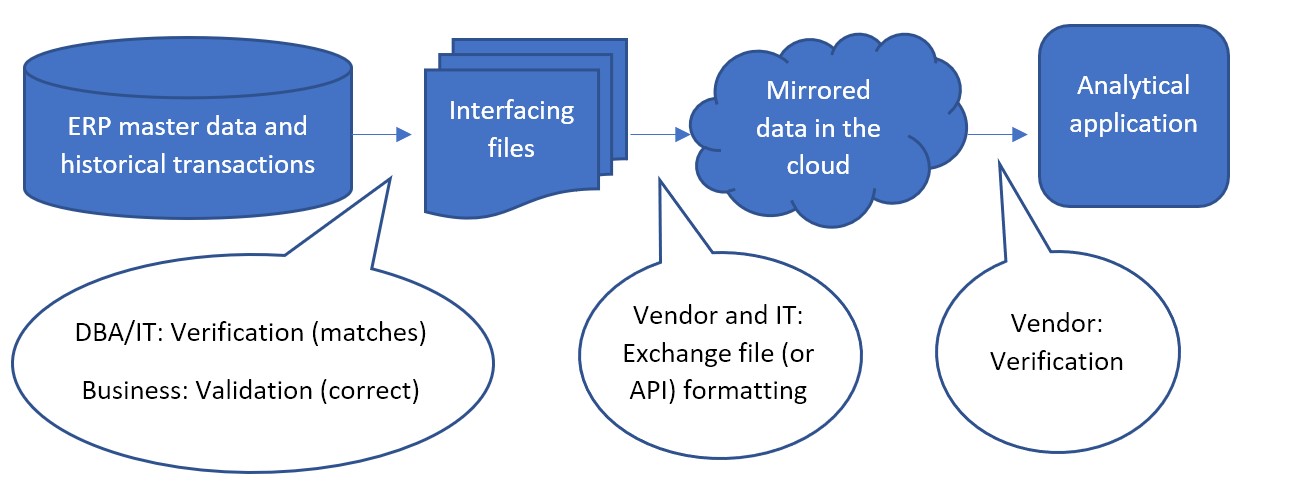
Epicor is Smarter
Epicor has partnered with Smart Software and offers Smart IP&O as a cross platform add-on to its ERP solutions including BisTrack, a speciality ERP for the Lumber, hardware, and building material industry.  The Smart IP&O solution comes complete with a bidirectional integration to BisTrack.  This enables Epicor customers to leverage built-for-purpose best of breed inventory optimization applications.  With Epicor Smart IP&O you can generate forecasts that capture trend and seasonality without manual configurations.  You will be able to automatically recalibrate inventory policies using field proven, cutting-edge statistical and probabilistic models that were engineered to accurately plan for intermittent demand.   Safety stocks will accurately account for demand and supply variability, business conditions, and priorities.  You can leverage service level driven planning so you have just enough stock or turn on optimization methods that prescribe the most profitable stocking policies and service levels that consider the real cost of carrying inventory. You can support commodity buys with accurate demand forecasting over longer horizons, and run “what-if” scenarios to assess alternative strategies before execution of the plan.

Smart IP&O customers routinely realize 7 figure annual returns from reduced expedites, increased sales, and less excess stock, all the while gaining a competitive edge by differentiating themselves on improved customer service. To see a recorded webinar hosted by the Epicor Users Group that profiles Smart’s Demand Planning and Inventory Optimization platform, please register here.

Sometimes a statistical forecast just doesn’t make sense.  Every forecaster has been there.  They may double-check that the data was input correctly or review the model settings but are still left scratching their head over why the forecast looks very unlike the demand history.   When the occasional forecast doesn’t make sense, it can erode confidence in the entire statistical forecasting process.

This blog will help a layman understand what the Smart statistical models are and how they are chosen automatically.  It will address how that choice sometimes fails, how you can know if it did, and what you can do to ensure that the forecasts can always be justified.  It’s important to know to expect, and how to catch the exceptions so you can rely on your forecasting system.

How methods are chosen automatically

The criteria to automatically choose one statistical method out of a set is based on which method came closest to correctly predicting held-out history.  Earlier history is passed to each method and the result is compared to actuals to find the one that came closest overall.  That automatically chosen method is then fed all the history to produce the forecast. Check out this blog to learn more about the model selection https://smartcorp.com/uncategorized/statistical-forecasting-how-automatic-method-selection-works/

For most time series, this process can capture trends, seasonality, and average volume accurately. But sometimes a chosen method comes mathematically closest to predicting the held-out history but doesn’t project it forward in a way that makes sense.  That means the system selected method isn’t best and for some “hard to forecast”

Hard to forecast items

Hard to forecast items may have large, unpredictable spikes in demand, or typically no demand but random irregular blips, or unusual recent activity.  Noise in the data sometimes randomly wanders up or down, and the automated best-pick method might forecast a runaway trend or a grind into zero.  It will do worse than common sense and in a small percentage of any reasonably varied group of items.  So, you will need to identify these cases and respond by overriding the forecast or changing the forecast inputs.

How to find the exceptions

Best practice is to filter or sort the forecasted items to identify those where the sum of the forecast over the next year is significantly different than the corresponding history last year.  The forecast sum may be much lower than the history or vice versa.  Use supplied metrics to identify these items; then you can choose to apply overrides to the forecast or modify the forecast settings.

How to fix the exceptions

Often when the forecast seems odd, an averaging method, like Single Exponential Smoothing or even a simple average using Freestyle, will produce a more reasonable forecast.  If trend is possibly valid, you can remove only seasonal methods to avoid a falsely seasonal result.  Or do the opposite and use only seasonal methods if seasonality is expected but wasn’t projected in the default forecast.  You can use the what-if features to create any number of forecasts, evaluate & compare, and continue to fine tune the settings until you are comfortable with the forecast.

Cleaning the history, with or without changing the automatic method selection, is also effective at producing reasonable forecasts. You can embed forecast parameters to reduce the amount of history used to forecast those items or the number of periods passed into the algorithm so earlier, outdated history is no longer considered.  You can edit spikes or drops in the demand history that are known anomalies so they don’t influence the outcome.  You can also work with the Smart team to implement automatic outlier detection and removal so that data prior to being forecasted is already cleansed of these anomalies.

If the demand is truly intermittent, it is going to be nearly impossible to forecast “accurately” per period. If a level-loading average is not acceptable, handling the item by setting inventory policy with a lead time forecast can be effective.  Alternatively, you may choose to use “same as last year” models which while not prone to accuracy will be generally accepted by the business given the alternatives forecasts.

Finally, if the item was introduced so recently that the algorithms do not have enough input to accurately forecast, a simple average or manual forecast may be best.  You can identify new items by filtering on the number of historical periods.

Manual selection of methods

Once you have identified rows where the forecast doesn’t make sense to the human eye, you can choose a smaller subset of all methods to allow into the forecast run and compare to history.  Smart will allow you to use a restricted set of methods just for one forecast run or embed the restricted set to use for all forecast runs going forward. Different methods will project the history into the future in different ways.  Having a sense of how each works will help you choose which to allow.

Rely on your forecasting tool

The more you use Smart period over period to embed your decisions about how to forecast and what historical data to consider, the less often you will face exceptions as described in this blog.  Entering forecast parameters is a manageable task when starting with critical or high impact items.  Even if you don’t embed any manual decisions on forecast methods, the forecast re-runs every period with new data. So, an item with an odd result today can become easily forecastable in time.

Service-Level-Driven Service Parts Planning for Microsoft Dynamics BC or F&SC is a four-step process that extends beyond simplified forecasting and rule-of-thumb safety stocks. It provides service parts planners with data-driven, risk-adjusted decision support.

The math to determine this level of planning simply does not exist in D365 functionality.  It requires math and AI that passes thousands of times through calculations for each part and part center (locations).  Math and AI like this are unique to Smart.  To understand more, please read on. 

Step 1. Ensure that all stakeholders agree on the metrics that matter. 

All participants in the service parts inventory planning process must agree on the definitions and what metrics matter most to the organization. Service Levels detail the percentage of time you can completely satisfy required usage without stocking out. Fill Rates detail the percentage of the requested usage that is immediately filled from stock. (To learn more about the differences between service levels and fill rate, watch this 4-minute lesson here.) Availability details the percentage of active spare parts with an on-hand inventory of at least one unit. Holding costs are the annualized costs of holding stock accounting for obsolescence, taxes, interest, warehousing, and other expenses. Shortage costs are the cost of running out of stock, including vehicle/equipment downtime, expedites, lost sales, and more. Ordering costs are the costs associated with placing and receiving replenishment orders.

Step 2. Benchmark historical and predicted current service level performance.

All participants in the service parts inventory planning process must hold a common understanding of predicted future service levels, fill rates, and costs and their implications for your service parts operations. It is critical to measure both historical Key Performance Indicators (KPIs) and their predictive equivalents, Key Performance Predictions (KPPs).  Leveraging modern software, you can benchmark past performance and leverage probabilistic forecasting methods to simulate future performance.  Virtually every Demand Planning solution stops here.  Smart goes further by stress-testing your current inventory stocking policies against all plausible future demand scenarios.  It is these thousands of calculations that build our KPPs.  The accuracy of this improves D365’s ability to balance the costs of holding too much with the costs of not having enough. You will know ahead of time how current and proposed stocking policies are likely to perform.

Step 3. Agree on targeted service levels for each spare part and take proactive corrective action when targets are predicted to miss. 

Parts planners, supply chain leadership, and the mechanical/maintenance teams should agree on the desired service level targets with a full understanding of the tradeoffs between stockout risk and inventory cost.  A call out here is that our D365 customers are almost always stunned by the stocking levels difference between 100% and 99.5% availability.   With the logic for nearly 10,000 scenarios that half a percent outage is almost never hit.   You achieve full stocking policy with much lower costs.   You find the parts that are understocked and correct those.  The balancing point is often a 7-12% reduction in inventory costs. 

This leveraging of what-if scenarios in our parts planning software gives management and buyers the ability to easily compare alternative stocking policies and identify those that best meet business objectives.  For some parts, a small stock out is okay.  For others, we need that 99.5% parts availability.  Once these limits are agreed upon, we use the Power of D365 to optimize inventory using D365 core ERP as it should be.   The planning is automatically uploaded to engage Dynamics with modified reorder points, safety stock levels, and/or Min/Max parameters.  This supports a single Enterprise center point, and people are not using multiple systems for their daily parts management and purchasing.

Step 4. Make it so and keep it so. 

Empower the planning team with the knowledge and tools it needs to ensure that you strike agreed-upon balance between service levels and costs.  This is critical and important.  Using Dynamics F&SC or BC to execute your ERP transactions is also important.  These two Dynamics ERPs have the highest level of new ERP growth on the planet.  Using them as they are intended to be used makes sense.   Filling the white space for the math and AI calculations for Maintenance and Parts management also makes sense.  This requires a more complex and targeted solution to help.  Smart Software Inventory Optimization for EAM and Dynamics ERPs holds the answer.    

Remember: Recalibration of your service parts inventory policy is preventive maintenance against both stockouts and excess stock.  It helps costs, frees capital for other uses, and supports best practices for your team. 

Extend Microsoft 365 F&SC and AX with Smart IP&O

To see a recording of the Microsoft Dynamics Communities Webinar showcasing Smart IP&O, register here:

https://smartcorp.com/inventory-planning-with-microsoft-365-fsc-and-ax/

Data verification and validation are essential to the success of the implementation of software that performs statistical analysis of data, like Smart IP&O.  This article describes the issue and serves as a practical guide to doing the job right, especially for the user of the new application.

The less experience your organization has in validating historical transactions or item master attributes, the more likely it is there were problems or mistakes with data entry into the ERP that have so far gone unnoticed.  The garbage in, garbage out rule means you need to prioritize this step of the software onboarding process or risk delay and possible failure to generate ROI.

Ultimately the best person to confirm data in your ERP is entered correctly is the person who knows the business and can assert, for example, “this part doesn’t belong to that product group.”  That’s usually the same person who will open and use Smart. Though a database administrator or IT support can also play a key role by being able to say, “This part was assigned to that product group last December by Jane Smith.” Ensuring data is correct may not be a regular part of your day job but can be broken down into manageable small tasks that a good project manager will allocate the time and resources to complete.

The demand planning software vendor receiving the data also has a role.  They will confirm that the raw data was ingested without issue. The vendor can also identify abnormalities in the raw data files that point to the need for validation.  But relying on the software vendor to reassure you the data looks fine is not enough.  You don’t want to discover, after go-live, that you can’t trust the output because some of the data “doesn’t make sense.”

Each step in the data flow needs verification and validation.  Verification means the data at one step is still the same after flowing to the next step.  Validation means the data is correct and usable for analysis. 

The most common data flow looks like this:

Less commonly, the first step between ERP master data and the interfacing files can sometimes be bypassed, where files are not used as an interface.  Instead, an API built by IT or the inventory optimization software vendor is responsible for data to be written directly from the ERP to the mirrored database in the cloud.  The vendor would work with IT to confirm the API is working as expected.  But the first validation step, even in that case, can still be performed.  After ingesting the data, the vendor can make the mirrored data available in files for the DBA/IT verification and business validation.

The confirmation that the mirrored data in the cloud completes the flow into the application is the responsibility of the vendor of software as a service.  SaaS vendors continually test that the software works correctly between the front-end application their subscribers see and the back-end data in the cloud database. If the subscribers still think the data doesn’t make sense in the application even after validating the interfacing files before going live, that is an issue to raise with the vendor’s customer support.

However the interfacing files are obtained, the largest part of verification and validation falls to the project manager and their team.  They must resource a test of the interfacing files to confirm:

1. They match the data in the ERP. And that all and only the ERP data that was necessary to extract for use in the application was extracted.
2. Nothing “jumps out” to the business as incorrect for each of the types of information in the data
3. They are formatted as expected.

DBA/IT Verification Tasks

1. Test the extract:

IT’s verification step can be done with various tools, comparing files, or importing files back to the database as temporary tables and joining them with the original data to confirm a match.  IT can depend on a query to pull the requested data into a file but that file can fail to match. The existence of delimiters or line returns within the data values can cause a file to be different than its original database table.  It is because the file relies heavily on delimiters and line returns to identify fields and records, while the table doesn’t rely on those characters to define its structure.

2. No bad characters:

Free form data entry fields in the ERP, such as product descriptions, can sometimes themselves contain line returns, tabs, commas, and/or double quotes that can affect the structure of the output file.  Line returns should not be allowed in values that will be extracted to a file.  Characters equal to the delimiter should be stripped during extract or else a different delimiter used.

Tip: if commas are the file delimiter, numbers greater than 999 can’t be extracted with a comma. Use “1000” rather than “1,000”.

3. Confirm the filters:

The other way that query extracts can return unexpected results is if conditions on the query are entered incorrectly.  The simplest way to avoid mistaken “where clauses” is to not use them.  Extract all data and allow the vendor to filter out some records according to rules supplied by the business.  If this will produce extract files so large that too much computing time is spent on the data exchange, the DBA/IT team should meet with the business to confirm exactly what filters on the data can be applied to avoid exchanging records that are meaningless to the application.

Tip: Bear in mind that Active/Inactive or item lifecycle information should not be used to filter out records.  This information should be sent to the application so it knows when an item becomes inactive.

4. Be consistent:

The extract process must produce files of consistent format every time it is executed.  File names, field names, and position, delimiter, and Excel sheet name if Excel is used, numeric formats and date formats, and the use of quotes around values should never differ from one execution of the extract one day to the next. A hands-off report or stored procedure should be prepared and used for every execution of the extract.

Business Validation Background

Below is a break down each of validation step into considerations, specifically in the case where the vendor has provided a template format for the interfacing files where each type of information is provided in its own file.  Files sent from your ERP to Smart are formatted for easy export from the ERP.  That sort of format makes the comparison back to the ERP a relatively simple job for IT, but it can be harder for the business to interpret.  Best practice is to manipulate the ERP data, either by using pivot tables or similar in a spreadsheet.  IT may assist by providing re-formatted data files for review by the business.

To delve into the interfacing files, you’ll need to understand them.  The vendor will supply a precise template, but generally interfacing files consist into three types: catalog data, item attributes, and transactional data.

• Catalog data contains identifiers and their attributes. Identifiers are typically for products, locations (which could be plants or warehouses), your customers, and your suppliers.
• Item attributes contain information about products at locations that are needed for analysis on the product and location combination. Such as:
  • Current replenishment policy in the form of a Min and Max, Reorder Point, or Review Period and Order Up To value, or Safety Stock
  • Primary supplier assignment and nominal lead time and cost per unit from that supplier
  • Order quantity requirements such as minimum order quantity, manufacturing lot size, or order multiples
  • Active/Inactive status of the product/location combination or flags that identify its state in its lifecycle, such as pre-obsolete
  • Attributes for grouping or filtering, such as assigned buyer/planner or product category
  • Current inventory information like on hand, on order, and in transit quantities.
• Transactional data contains references to identifiers along with dates and quantities. Such as quantity sold in a sales order of a product, at a location, for a customer, on a date.  Or quantity placed on purchase order of a product, into a location, from a supplier, on a date. Or quantity used in a work order of a component product at a location on a date.

Validating Catalog Data

Considering catalog data first, you may have catalog files similar to these examples:

1: Check for a reasonable count of catalog records

For each file of catalog data, open it in a spreadsheet tool like Google Sheets or MS Excel. Answer these questions:

1. Is the record count in the ballpark? If you have about 50K products, there should not be only 10K rows in its file.
2. If it’s a short file, maybe the Location file, you can confirm exactly that all expected Iidentifiers are in it.
3. Filter by each attribute value and confirm again the count of records with that attribute value makes sense.

2: Check the correctness of values in each attribute field

Someone who knows what the products are and what the groups mean needs to take the time to confirm it is actually right, for all the attributes of all the catalog data.

So, if your Product file contains the attributes as in the example above, you would filter for Status of Active, and check that all resulting products are actually active.  Then filter for Status of Inactive and check that all resulting products are actually inactive.  Then filter for the first Group value and confirm all resulting products are in that group.  Repeat for Group2 and Group3, etc.  Then repeat for every attribute in every file.

It can help to do this validation with a comparison to an already existing and trusted report.  If you have another spreadsheet that shows products by Group for any reason, you can compare the interfacing files to it.  You may need to familiarize yourself with the VLOOKUP function that helps with spreadsheet comparison.

Validating Item Attribute Data

1: Check for a reasonable count of item records

The item attribute data confirmation is similar to the catalog data.  Confirm the product/location combination count makes sense in total and for each of the unique item attributes, one by one. This is an example item data file:

2: Find and explain weird numbers in item file

There tends to be many numerical values in the item attributes, so “weird” numbers merit review.  To validate data for a numerical attribute in any file, search for where the number is:

• Missing entirely
• Equal to zero
• Less than zero
• More than most others, or less than most others (sort by that column)
• Not a number at all, when it should be

A special consideration of files that are not catalog files is they may not show the descriptions of the products and locations, just their identifiers, which can be meaningless to you.  You can insert columns to hold the product and location descriptors that you are used to seeing and fill them into the spreadsheet to assist in your work.  The VLOOKUP function works for this as well.  Whether or not you have another report to compare the Items file to, you have the catalog files for Products and Location with show both the identifier and the description for each row.

3: Spot check

If you are frustrated to find that there are too many attribute values to manually check in a reasonable amount of time, spot checking is a solution. It can be done in a manner likely to pick up on any problems.  For each attribute, get a list of the unique values in each column.  You can copy a column into a new sheet, then use the Remove Duplicates function to see the list of possible values.   With it:

1. Confirm that no attribute values are present that shouldn’t be.
2. It can be harder to remember which attribute values are missing that should be there, so it can help to look at another source to remind you. For example, if Group1 through Group12 are present, you might check another source to remember if these are all the Groups possible.  Even if it is not required for the interfacing files for the application, it may be easy for IT to extract a list of all the possible Groups that are in your ERP which you can use for the validation exercise.  If you find extra or missing values that you don’t expect, bring an example of each to IT to investigate.
3. Sort alphabetically and scan down to see if any two values are similar but slightly different, maybe only in punctuation, which could mean one record had the attribute data entered incorrectly.

For each type of item, maybe one from each product group and/or location, check that all its attributes in every file are correct or at least pass a sanity check.  The more you can spot check from a broad range of items, the less likely you will have issues post go live.

Validating Transactional Data

Transactional files may all have a format similar to this:

1: Find and explain weird numbers in each transactional file

These should be checked for “weird” numbers in the Quantity field.  Then you can proceed to:

1. Filter for dates outside the range you expect or missing expected dates entirely.
2. Find where Transaction identifiers and line numbers are missing. They shouldn’t be.
3. If there is more than one record for a given Transaction ID and Transaction Line Number combination, is that a mistake? Put another way, should duplicate records have their quantities summed together or is that double counting?

2: Sanity check summed quantities

Do a sanity check by filtering to a particular product you’re familiar with, and filter to a relatable date range such as last month or last year, and sum the quantities.  Is that total amount what you expected for that product in that time frame?  If you have information on total usage out of a location, you can slice the data that way to sum the quantities and compare to what you expect.  Pivot tables come in handy for verification of transactional data.  With them, you can view the data like:

The products’ yearly total may be simple to sanity check if you know the products well.  Or you can VLOOKUP to add attributes, such as product group, and pivot on that to see a higher level that is more familiar:

3: Sanity check count of records

It may help to display a count of transactions rather than a sum of the quantities, especially for purchase order data.  Such as:

And/or the same summarization at a higher level, like:

4: Spot checking

Spot checking the correctness of a single transaction, for each type of item and each type of transaction, completes due diligence.  Pay special attention to what date is tied to the transaction, and whether it is right for the analysis.  Dates may be a creation date, like the date a customer placed an order with you, or a promise date, like the date you expected to deliver on the customer’s order at the time of creating it, or a fulfilment date, when you actually delivered on the order.  Sometimes a promise date gets modified days after creating the order if it can’t be met.  Make sure the date in use reflects actual demand by the customer for the product most closely.

What to do about bad data 

If the mis-entries are few or one-off, you can edit the ERP records by hand as they are found, cleaning up your catalog attributes, even after go-live with the application.  But if large swathes of attributes or transaction quantities are off, this can spur an internal project to re-enter data correctly and possibly to change or start to document the process that needs to be followed when new records are entered into your ERP.

Care must be taken to avoid too long a delay in implementation of the SaaS application while waiting on clean attributes.  Break the work into chunks and use the application to analyze the clean data first so the data cleansing project occurs in parallel with getting value out of the new application.

Smart IP&O offers automated statistical forecasting that selects the right forecast method that best forecasts the data.  It does this for each time-series in the data set.  This blog will help a laymen understand how the forecast methods are chosen automatically.

Smart makes many methods available including single and double exponential smoothing, linear and simple moving average, and Winters models.  Each model is designed to capture a different sort of pattern.  The criteria to automatically choose one statistical method out of a set of choices is based on which method came closest to correctly predicting held-out history.

Earlier demand history is passed to each method and the result is compared to actuals to find the one that came closest overall.  That “winning” automatically chosen method is then fed all the history for that item to produce the forecast.

The overall nature of the demand pattern for the item is captured by holding out different portions of the history so that an occasional outlier does not unduly influence the choice of method.  You can visualize it using the below diagram where each row represents a 3-period forecast in held out history, based on different amounts of the red earlier history.  The variances of each pass are averaged together to determine the method’s overall ranking against all other methods.

For most time series, this process can accurately capture trends, seasonality, and average volume accurately. But sometimes a chosen method comes mathematically closest to predicting the held-out history but doesn’t project it forward in a way that makes sense.

Users can correct this by using the system’s exception reports and filtering features to identify items that merit review.  They can then configure the automatic forecast methods that they wish to be considered for that item.