The promise of a digital supply chain has transformed how businesses operate. At its core, it can make rapid, data-driven decisions while ensuring quality and efficiency throughout operations. However, it’s not just about having access to more data. Organizations need the right tools and platforms to turn that data into actionable insights. This is where decision-making becomes critical, especially in a landscape where new digital supply chain solutions and AI-driven platforms can support you in streamlining many processes within the decision matrix.

Why Is Rapid Decision-Making in the Digital Supply Chain So Important?

Business is accelerating; customers expect faster delivery, higher service levels, and greater transparency. The key to meeting these demands lies in digital supply chain solutions that support decision intelligence.

Yet, many organizations struggle. The gap between data, analytics, and action persists. Businesses gather vast amounts of information but fail to act on it quickly enough, or worse, they make decisions based on outdated or incomplete data. Bridging this gap is necessary for realizing the true value of a digital supply chain.

Rapid Decision-Making and Quality Implications

1. The Decision Gap
Many organizations are stuck between collecting data and acting. This “decision gap” causes delays, reducing the potential business value that could have been realized. In a supply chain setting, delayed decisions can lead to stockouts, overstocking, lost sales, and dissatisfied customers.

2. New AI Platforms Are Key
Digital and AI platforms enable businesses to make quicker, more informed decisions by digitizing the data-to-action process. Demand Forecasting and Inventory Optimization are key processes within the decision matrix, and tools like Smart IP&O help predict inventory needs and optimize those decisions based on cost, service levels, and changing demand patterns. This allows for decision-making at a speed and scale previously unachievable. Additionally, Smart IP&O supports more significant strategic decisions and smaller, more frequent operational decisions, ensuring a wide range of the supply chain is optimized.

3. Quality of Decision-Making
Rapid decisions alone aren’t enough. The quality of those decisions matters.   Effective decision-making requires accurate data, forecasting, and analysis to ensure that decisions lead to positive outcomes. Organizations can better balance important factors like cost, availability, and service levels by leveraging tools that provide insights into future trends and performance. This approach allows them to create strategies aligned with actual needs and demands, improving efficiency and overall success.

Smart IP&O uses advanced forecasting models and real-time data to ensure quick and reliable decisions. For example, organizations can use projected metrics to balance service levels, costs, and stock availability, ensuring inventory policies align with actual demand trends​​.

4. Scalability and Consistency in Decision-Making
As businesses grow, the complexity of supply chain decisions increases, and handling an increasing number of products, data points, and processes can be challenging. Digital platforms and automation tools help businesses scale their decision-making processes by managing vast amounts of data with precision and uniformity.

By automating repetitive tasks and applying consistent rules across various scenarios, businesses can ensure that decisions are made uniformly, leading to more predictable and reliable outcomes​​. This approach leads to more predictable and reliable outcomes, as automated systems ensure that decisions are consistent even as the business expands.

AI driven platforms like Smart IP&O offer scalability, allowing businesses to manage thousands of products and data points with constant accuracy. This consistency is critical in maintaining service levels and reducing costs as operations expand.

5. Digitization of Decision Processes
Digitization of decision processes involves automating various aspects of decision-making. By using digital tools, routine decisions—such as those related to inventory, demand, and production—can be automated, allowing for faster and more efficient handling of day-to-day tasks. In cases where human intervention is still required, systems can be set up to notify users when specific conditions or thresholds are met. This reduces manual effort and enables employees to focus on more strategic and complex work, ultimately enhancing productivity and efficiency.

 

The promise of the digital supply chain lies in its ability to transform data into action quickly and accurately. To fully capitalize on this promise, organizations need to bridge the decision gap by adopting platforms like Smart IP&O. These platforms enhance rapid decision-making and ensure that quality isn’t sacrificed in the process. As businesses evolve, those that successfully integrate these tools into their decision matrix will be better positioned to stay competitive and meet ever-growing customer expectations.

 

Demand planning goes beyond simply forecasting product needs; it’s about ensuring your business meets customer demands with precision, efficiency, and cost-effectiveness. Latest demand planning technology addresses key challenges like forecast accuracy, inventory management, and market responsiveness. In this blog, we will introduce critical demand planning trends, including data-driven insights, probabilistic forecasting, consensus planning, predictive analytics, scenario modeling, real-time visibility, and multilevel forecasting. These trends will help you stay ahead of the curve, optimize your supply chain, reduce costs, and enhance customer satisfaction, positioning your business for long-term success.

Data-Driven Insights

Advanced analytics, machine learning, and artificial intelligence (AI) are becoming integral to demand planning. Technologies like Smart UP&O allow businesses to analyze complex data sets, identify patterns, and make more accurate predictions. This shift towards data-driven insights helps businesses respond quickly to market changes, minimizing stockouts and reducing excess inventory.

Probabilistic Forecasting

Probabilistic forecasting focuses on predicting a range of possible outcomes rather than a single figure. This trend is particularly important for managing uncertainty and risk in demand planning. It helps businesses prepare for various demand scenarios, enhancing inventory management and reducing the likelihood of stockouts or overstocking​.

Consensus Forecasting

Modern manufacturing is moving towards an integrated approach where departments and stakeholders collaborate more closely. Collaborative forecasting involves sharing insights across the supply chain, from suppliers to distributors and internal teams. This approach breaks down silos and ensures that everyone is working towards a common goal, leading to a more synchronized and efficient supply chain​.

Predictive and Prescriptive Analytics

Predictive analytics forecasts future outcomes based on historical data and trends, helping businesses anticipate demand fluctuations. For example, Smart Demand Planner (SDP) automates forecasting to adjust inventory and production levels accordingly​.

Prescriptive analytics goes further by offering actionable recommendations. Smart Inventory Planning and Optimization (IP&O), for instance, prescribes optimal inventory policies based on service levels, costs, and risks​. ogether, these tools enable proactive decision-making, allowing companies to both predict and optimize their responses to future challenges.

Scenario Modeling

Scenario modeling is becoming a key part of demand planning, enabling businesses to simulate different scenarios and assess their impact on operations. This method helps companies create adaptable strategies to effectively handle uncertainties. Smart IP&O enhances this capability by offering What If Scenarios that allow users to test different inventory policies before implementation. By adjusting variables like service levels or order quantities, businesses can visualize the effects on costs and service levels, empowering them to select the optimal strategy for minimizing risks and controlling costs​​.

Real-Time Visibility

As supply chains become more global and interconnected, real-time visibility into inventory and supply chain activities is crucial. Enhanced collaboration with suppliers and distributors, combined with real-time data, enables businesses to make quicker, more informed decisions. This helps optimize inventory levels, reduce lead times, and improve overall supply chain resilience​.

Multilevel Forecasting

This involves forecasting at different levels of the product hierarchy, such as individual items, product families, or even entire product lines. Multilevel forecasting is vital for businesses with complex product portfolios, as it ensures that forecasts are accurate at both the micro and macro levels​.

 

Demand planning is a decisive aspect of modern supply chain management, offering businesses the ability to enhance operational efficiency, reduce costs, and better meet customer demands. Leveraging advanced platforms like Smart IP&O significantly improves forecasting accuracy and inventory management, enabling swift responses to market fluctuations. Automated statistical forecasting, combined with capabilities like hierarchy forecasting and forecast overrides, ensures that forecasts are accurate and adaptable, leading to more realistic planning decisions. Additionally, with tools like scenario modeling, businesses can explore various demand scenarios across their product hierarchy, facilitating informed decision-making by providing insights into potential outcomes and risks. This approach allows businesses to anticipate the impact of policy changes, make better decisions, and ultimately optimize their inventory and overall supply chain management, staying ahead of key trends in the process.

 

 

 

In this blog, we will analyze the automatic forecasting for time series demand projections, focusing on key techniques, challenges, and best practices. There are multiple methods to predict future demand for an item, and this becomes complex when dealing with thousands of items, each requiring a different forecasting technique due to their unique demand patterns. Some items have stable demand, others trend upwards or downwards, and some exhibit seasonality. Selecting the right method for each item can be overwhelming. Here, we’ll explore how automatic forecasting simplifies this process.

Automatic forecasting becomes fundamental in managing large-scale demand projections. With thousands of items, manually selecting a forecasting method for each is impractical. Automatic forecasting uses software to make these decisions, ensuring accuracy and efficiency in the forecasting process. It’s importance lies in its ability to handle complex, large-scale forecasting needs efficiently. It eliminates the need for manual selection, saving time and reducing errors. This approach is particularly beneficial in environments with diverse demand patterns, where each item may require a different forecasting method.

 

Key Considerations for Effective Forecasting

1. Challenges of Manual Forecasting:
   • Infeasibility: Manually choosing forecasting methods for thousands of items is unmanageable.
   • Inconsistency: Human error can lead to inconsistent and inaccurate forecasts.
2. Criteria for Method Selection:
   • Error Measurement: The primary criterion for selecting a forecasting method is the typical forecast error, defined as the difference between predicted and actual values. This error is averaged over the forecast horizon (e.g., monthly forecasts over a year).
   • Holdout Analysis: This technique simulates the process of waiting for a year to elapse by hiding some historical data, making forecasts, and then revealing the hidden data to compute errors. This helps in choosing the best method in real-time.
3. Forecasting Tournament:
   • Method Comparison: Different methods compete to forecast each item, with the method producing the lowest average error winning.
   • Parameter Tuning: Each method is tested with various parameters to find the optimal settings. For example, simple exponential smoothing may be tried with different weighting factors.

 

The Algorithms Behind Effective Automatic Forecasting

Automatic forecasting is highly computational but feasible with modern technology. The process involves:

• Data Segmentation: Dividing historical data into segments helps manage and leverage different aspects of historical data for more accurate forecasting. For instance, for a product with seasonal demand, data might be segmented by seasons to capture season-specific trends and patterns. This segmentation allows forecasters to make and test forecasts more effectively.
• Repeated Simulations: Using sliding simulations involves repeatedly testing and refining forecasts over different periods. This method validates the accuracy of forecasting methods by applying them to different segments of data. An example is the sliding window method, where a fixed-size window moves across the time series data, generating forecasts for each position to evaluate performance.
• Parameter Optimization: Parameter optimization involves trying multiple variants of each forecasting method to find the best-performing one. By adjusting parameters, such as the smoothing factor in exponential smoothing methods or the number of past observations in ARIMA models, forecasters can fine-tune models to improve performance.

For instance, in our software, we allow various forecasting methods to compete for the best performance on a given item.  Knowledge of Automatic forecasting immediately carries over to Simple Moving Average, linear moving average, Single Exponential Smoothing, Double Exponential Smoothing, Winters’ Exponential Smoothing, and Promo forecasting. This competition ensures that the most suitable method is selected based on empirical evidence, not subjective judgment. The tournament winner is the closest method to predicting new data values from old. Accuracy is measured by average absolute error (that is, the average error, ignoring any minus signs). The average is computed over a set of forecasts, each using a portion of the data, in a process known as sliding simulation, which we have explained previously in a previous blog.

 

Methods used in Automatic forecasting

Normally, there are six extrapolative forecasting methods competing in the Automatic forecasting tournament:

• Simple moving average
• Linear moving average
• Single exponential smoothing
• Double exponential smoothing
• Additive version of Winters’ exponential smoothing
• Multiplicative version of Winters’ exponential smoothing

The latter two methods are appropriate for seasonal series; however, they are automatically excluded from the tournament if there are fewer than two full seasonal cycles of data (for example, fewer than 24 periods of monthly data or eight periods of quarterly data). These six classical, smoothing-based methods have proven themselves to be easy to understand, easy to compute and accurate. You can exclude any of these methods from the tournament if you have a preference for some of the competitors and not others.

Automatic forecasting for time series data is essential for managing large-scale demand projections efficiently and accurately. Businesses can achieve better forecast accuracy and streamline their planning processes by automating the selection of forecasting methods and utilizing techniques like holdout analysis and forecasting tournaments. Embracing these advanced forecasting techniques ensures that businesses stay ahead in dynamic market environments, making informed decisions based on reliable data projections.

 

 

 

In this blog, we will explore how organizations can achieve exceptional efficiency and accuracy with AI-driven inventory optimization. Traditional inventory management methods often fall short due to their reactive nature and reliance on manual processes. Maintaining optimal inventory levels is fundamental for meeting customer demand while minimizing costs. The introduction of AI-driven inventory optimization can significantly reduce the burden of manual processes, providing relief to supply chain managers from tedious tasks. With AI, we can predict demand more accurately, reduce excess stock, avoid stockouts, and ultimately improve our organization’s bottom line. Let’s explore how this approach not only boosts sales and operational efficiency but also elevates customer satisfaction by ensuring products are always available when needed.

 

Insights for Improved Decision-Making in Inventory Management

1. Enhanced Forecast Accuracy Advanced Machine Learning algorithms analyze historical data to identify patterns that humans might miss. Techniques like clustering, regime change detection, anomaly detection, and regression analysis provide deep insights into data. Measuring forecast error is essential for refining forecast models; for example, techniques like Mean Absolute Error (MAE) and Root Mean Squared Error (RMSE) help quantify the accuracy of forecasts. Businesses can improve accuracy by continuously monitoring and adjusting forecasts based on these error metrics. As the Demand Planner at a Hardware Retailer stated, “With the improvements to our forecasts and inventory planning that Smart Software enabled, we have been able to reduce safety stock by 20% while also reducing stock-outs by 35%.”

2. Real-Time Data Analysis State-of-the-art systems can process vast amounts of data in real time, allowing businesses to adjust their inventory levels dynamically based on current demand trends and market conditions. Anomaly detection algorithms can automatically identify and correct sudden spikes or drops in demand, ensuring that the forecasts remain accurate. A notable success story comes from Smart IP&O, which enabled one company to reduce inventory by 20% while maintaining service levels by continuously analyzing real-time data and adjusting forecasts accordingly. FedEx Tech’s Manager of Materials highlighted, “Whatever the request, we need to meet our next-day service commitment – Smart enables us to risk adjust our inventory to be sure we have the products and parts on hand to achieve the service levels our customers require.”

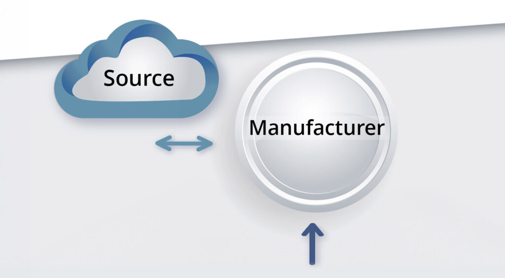
3. Improved Supply Chain Efficiency Intelligent technology platforms can optimize the entire supply chain, from procurement to distribution, by predicting lead times and optimizing order quantities. This reduces the risk of overstocking and understocking. For instance, using forecast-based inventory management, Smart Software helped a manufacturer streamline its supply chain, reducing lead times by 15% and enhancing overall efficiency. The VP of Operations at Procon Pump stated, “One of the things I like about this new tool… is that I can evaluate the consequences of inventory stocking decisions before I implement them.”

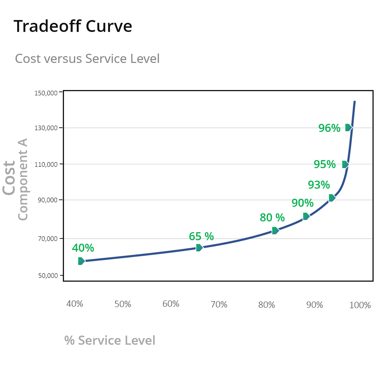
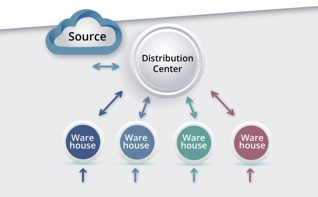
4. Enhanced Decision-Making AI provides actionable insights and recommendations, enabling managers to make informed decisions. This includes identifying slow-moving items, forecasting future demand, and optimizing stock levels. Regression analysis, for example, can relate sales to external variables like seasonality or economic indicators, providing a deeper understanding of demand drivers. One of Smart Software’s clients reported a significant improvement in decision-making processes, resulting in a 30% increase in service levels while reducing excess inventory by 15%. “Smart IP&O enabled us to model demand at each stocking location and, using service level-driven planning, determine how much to stock to achieve the service level we require,” noted the Purchasing Manager at Seneca Companies.

5. Cost Reduction By optimizing inventory levels, businesses can reduce holding costs and minimize losses from obsolete or expired products. AI-driven systems also reduce the need for manual inventory checks, saving time and labor costs. A recent case study shows how implementing Inventory Planning & Optimization (IP&O) was accomplished within 90 days of project start. Over the ensuing six months, IP&O enabled the adjustment of stocking parameters for several thousand items, resulting in inventory reductions of $9.0 million while sustaining target service levels.

 

By leveraging advanced algorithms and real-time data analysis, businesses can maintain optimal inventory levels and enhance their overall supply chain performance. Inventory Planning & Optimization (IP&O) is a powerful tool that can help your organization achieve these goals. Incorporating state-of-the-art inventory optimization into your organization can lead to significant improvements in efficiency, cost reduction, and customer satisfaction.

 

 

Utilities have unique supply chain optimization requirements, primarily ensuring high uptime by keeping all critical machines running continuously. Achieving this involves maintaining a high availability of spare parts to guarantee a consistent, reliable, and safe supply. Additionally, as regulated entities, utilities must also carefully manage and control costs.

Managing supply chains efficiently

To maintain a reliable electricity supply at 99.99%⁺ service levels, for example, utilities must be able to respond quickly to changes in demand in the near term and accurately anticipate future demand. To do so, they must have a well-organized supply chain that allows them to purchase the necessary equipment, materials, and services from the right suppliers at the right time, in the right quantities, and at the right price.

Doing so has become increasingly more challenging in the last 3 years.

• Requirements for safety, reliability, and service delivery are more stringent.
• Supply chain disruptions, unpredictable supplier lead times, intermittent spikes in parts usage have always been problematic, but now they are more the rule than the exception.
• Deregulation in the early 2000’s removed spare parts from the list of directly reimbursed items, forcing utilities to pay for spares directly from revenues[1]
• The constant need for capital combined with aggressively climbing interest rates mean costs are scrutinized more than ever.

As a result, Supply Chain Optimization (SCO) has become an increasingly mission-critical business practice for utilities.  To contend with these challenges, utilities can no longer simply manage their supply chain — they must optimize it.  And to do that, investments in new processes and systems will be required.

[1] Scala et al. “Risk and Spare Parts Inventory in Electric Utilities”. Proceedings of the Industrial Engineering Research Conference.

Inventory Planning and Optimization   

Targeted investments in inventory optimization technology offer a path forward for every utility.  Inventory Optimization solutions should be prioritized because they:

1. Can be implemented in a fraction of the time required for initiatives in other areas, such as warehouse management, supply chain design,  and procurement consolidations. It is not uncommon to start generating benefit after 90 days and to have a full software deployment in less than 180 days.
2. Can generate massive ROI, yielding 20x returns and seven figure financial benefits annually. By better forecasting parts usage, utilities will reduce costs by purchasing only the necessary inventory while controlling the risk of stockouts that lead to downtime and poor service levels.
3. Provide foundational support for other initiatives. A strong supply chain rests on the foundation of solid usage forecasts and inventory purchasing plans.

Using predictive analytics and advanced algorithms, inventory optimization helps utilities maximize service levels and reduce operational costs by optimizing inventory levels for spare parts. For example, an electric utility might use statistical forecasting to predict future parts usage, conduct inventory audits to identify excess inventory, and leverage analytical results to identify where inventory optimization efforts should focus first. By doing this, the utility can ensure that machines are running at optimal levels and reduce the risk of costly delays due to a lack of spares.

By using analytics and data, you can identify which spare parts and equipment are most likely to be needed and order only the necessary items. This helps to ensure that equipment has high up-time. It rewards regular monitoring and adjusting of inventory levels so that when operating conditions change, you can detect the change and adjust accordingly. This implies that planning cycles must operate at a tempo high enough to keep up with changing conditions. Leveraging probabilistic forecasting to recalibrate spares stocking policies for each planning cycle ensures that stocking policies (such as min/max levels) are always up-to-date and reflect the latest parts usage and supplier lead times.

 

Service Levels and the Tradeoff Curve

The Service Level Tradeoff Curve relates inventory investment to item availability as measured by service level. Service level is the probability that no shortages occur between when you order more stock and when it arrives on the shelf. Surprisingly few companies have data on this important metric across their whole fleet of spare parts.

The Service Level Tradeoff Curve exposes the link between the costs associated with different levels of service and the inventory requirements needed to achieve them.  Knowing which components are important to maintaining high service levels is key to the optimization process and is determined by several factors, including inventory item standardization, criticality, historical usage, and known future repair orders. By understanding this relationship, utilities can better allocate resources, as when using the curves to identify areas where costs can be reduced without hurting system reliability.

With inventory optimization software, setting stocking policies is pure guesswork: It is possible to know how any given increase or decrease will impact service levels other than rough cut estimates.  How the changes will play out in terms of inventory investment, operating costs, and shortage costs, is something no one really knows.  Most utilities rely on rule of thumb methods and arbitrarily adjust stocking policies in a reactive manner after something has gone wrong such as a large stockout or inventory write off.  When adjustments are made this way, there is no fact-based analysis detailing how this change is expected to impact the metrics that matter:  service levels and inventory values.

Inventory Optimization software can compute the detailed, quantitative tradeoff curves required to make informed inventory policy choices or even recommend the target service level that results in the lowest overall operating cost (the sum of holding, ordering, and stock-out costs).  Using this analysis, large increases in stock levels may be mathematically justified when the predicted reduction in shortage costs exceeds the increase in inventory investment and associated holding costs.  By setting appropriate service levels and recalibrating policies across all active parts once every planning cycle (at least once monthly), utilities can minimize the risk of outages while controlling expenditures.

Perhaps the most critical aspects of the response to equipment breakdown are those relating to achieving a first-time fix as rapidly as possible. Having the proper spares available can be the difference between completing a single trip and increasing the mean time to repair, bearing the costs associated with several visits, and causing customer relationships to degrade.

Using modern software, you can benchmark past performance and leverage probabilistic forecasting methods to simulate future performance. By stress-testing your current inventory stocking policies against all plausible scenarios of future parts usage, you will know ahead of time how current and proposed stocking policies are likely to perform. Check out our blog post on how to measure the accuracy of your service level forecast to help you assess the accuracy of inventory recommendations that software providers will purport to provide benefit.

 

 

Leveraging Advanced Analytics and AI

When introducing automation, each utility company has its own goals to pursue, but you should begin with assessing present operations to identify areas that may be made more effective. Some companies may prioritize financial issues, but others may prioritize regulatory demands such as clean energy spending or industry-wide changes such as smart grids. Each company’s difficulties are unique, but modern software can point the way to a more effective inventory management system that minimizes excess inventory and places the correct components in the right places at the right times.

Overall, Supply Chain Optimization initiatives are essential for utilities looking to maximize their efficiency and reduce their costs. Technology allows us to make the integration process seamless, and you don’t need to replace your current ERP or EAM system by doing it.  You just need to make better use of the data you already have.

For example, one large utility launched a strategic Supply Chain Optimization (SCO) initiative and added best-in-class capabilities through the selection and integration of commercial off-the-shelf applications.  Chief among these was the Smart Inventory Planning and Optimization system (Smart IP&O), comprising Parts Forecasting / Demand Planning and Inventory Optimization functionality. Within just 90 days the software system was up and running, soon reducing inventory by $9,000,000 while maintaining spares availability at a high level. You can read the case study here Electric Utility Goes with Smart IP&O.

Utilities can ensure that they are able to manage their spare parts supplies in an efficient and cost-effective manner better preparing them for the future.  Over time, this balance between supply and demand translates to a significant edge. Understanding the Service Level Tradeoff Curve helps to understand the costs associated with different levels of service and the inventory requirements needed to achieve them. This leads to reduced operational costs, optimized inventory, and assurance that you can meet your customers’ needs.