For most small-to-medium manufacturers and distributors, single-level or single-echelon inventory optimization is at the cutting edge of logistics practice. Multi-echelon inventory optimization (“MEIO”) involves playing the game at an even higher level and is therefore much less common. This blog is the first of two. It aims to explain what MEIO is, why standard MEIO theories break down, and how probabilistic modeling through scenario simulation can restore reality to the MEIO process. The second blog will show a particular example.

Definition of Inventory Optimization

An inventory system is built on a set of design choices.

The first choice is the policy for responding to stockouts: Do you just lose the sale to a competitor, or can you convince the customer to accept a backorder? The former is more common with distributors than manufacturers, but this may not be much of a choice since customers may dictate the answer.

The second choice is the inventory policy. These divide into “continuous review” and “periodic review” policies, with several options within each type. You can link to a video tutorial describing several common inventory policies here.  Perhaps the most efficient is known to practitioners as “Min/Max” and to academics as (s, S) or “little S, Big S.” We use this policy in the scenario simulations below. It works as follows: When on-hand inventory drops to or below the Min (s), an order is placed for replenishment. The size of the order is the gap between the on-hand inventory and the Max (S), so if Min is 10, Max is 25 and on-hand is 8, it’s time for an order of 25-8 = 17 units.

The third choice is to decide on the best values of the inventory policy “parameters”, e.g., the values to use for Min and Max. Before assigning numbers to Min and Max, you need clarity on what “best” means for you. Commonly, best means choices that minimize inventory operating costs subject to a floor on item availability, expressed either as Service Level or Fill Rate. In mathematical terms, this is a “two-dimensional constrained integer optimization problem”. “Two-dimensional” because you have to pick two numbers: Min and Max. “Integer” because Min and Max have to be whole numbers. “Constrained” because you must pick Min and Max values that give a high-enough level of item availability such as service levels and fill rates. “Optimization” because you  want to get there with the lowest operating cost (operating cost combines holding, ordering and shortage costs).

Multiechelon Inventory Systems

The optimization problem becomes more difficult in multi-echelon systems. In a single-echelon system, each inventory item can be analyzed in isolation: one pair of Min/Max values per SKU. Because there are more parts to a multiechelon system, there is a bigger computational problem.

Figure 1 shows a simple two-level system for managing a single SKU. At the lower level, demands arrive at multiple warehouses. When those are in danger of stocking out, they are resupplied from a distribution center (DC). When the DC itself is in danger of stocking out, it is supplied by some outside source, such as the manufacturer of the item.

The design problem here is multidimensional: We need Min and Max values for 4 warehouses and for the DC, so the optimization occurs in 4×2+1×2=10 dimensions. The analysis must take account of a multitude of contextual factors:

• The average level and volatility of demand coming into each warehouse.
• The average and variability of replenishment lead times from the DC.
• The average and variability of replenishment lead times from the source.
• The required minimum service level at the warehouses.
• The required minimum service level at the DC.
• The holding, ordering and shortage costs at each warehouse.
• The holding, ordering and shortage costs at the DC.

As you might expect, seat-of-the-pants guesses won’t do well in this situation. Neither will trying to simplify the problem by analyzing each echelon separately. For instance, stockouts at the DC increase the risk of stockouts at the warehouse level and vice versa.

This problem is obviously too complicated to try to solve without help from some sort of computer model.

Why Standard Inventory Theory is Bad Math

With a little looking, you can find models, journal articles and book about MEIO. These are valuable sources of information and insight, even numbers. But most of them rely on the expedient of over-simplifying the problem to make it possible to write and solve equations. This is the “Fantasy” referred to in the title.

Doing so is a classic modeling maneuver and is not necessarily a bad idea. When I was a graduate student at MIT, I was taught the value of having two models: a small, rough model to serve as a kind of sighting scope and a larger, more accurate model to produce reliable numbers. The smaller model is equation-based and theory-based; the bigger model is procedure-based and data-based, i.e., a detailed system simulation. Models based on simple theories and equations can produce bad numerical estimates and even miss whole phenomena. In contrast, models based on procedures (e.g., “order up to the Max when you breach the Min”) and facts (e.g., the last 3 years of daily item demand) will require a lot more computing but give more realistic answers. Luckily, thanks to the cloud, we have a lot of computing power at our fingertips.

Perhaps the greatest modeling “sin” in the MEIO literature is the assumption that demands at all echelons can be modeled as purely random Poisson processes. Even if it were true at the warehouse level, it would be far from true at the DC level. The Poisson process is the “white rat of demand modeling” because it is simple and permits more paper-and-pencil equation manipulation. Since not all demands are Poisson shaped, this results in unrealistic recommendations.

Scenario-based Simulation Optimization

To get realism, we must get down into the details of how the inventory systems operate at each echelon. With few limits except those imposed by hardware such as size of memory, computer programs can keep up any level of complexity. For instance, there is no need to assume that each of the warehouses faces identical demand streams or has the same costs as all the others.

A computer simulation works as follows.

1. The real-world demand history and lead time history are gathered for each SKU at each location.
2. Values of inventory parameters (e.g., Min and Max) are selected for trial.
3. The demand and replenishment histories are used to create scenarios depicting inputs to the computer program that encodes the rules of operation of the system.
4. The inputs are used to drive the operation of a computer model of the system with the chosen parameter values over a long period, say one year.
5. Key performance indicators (KPI’s) are calculated for the simulated year.
6. Steps 2-5 are repeated many times and the results averaged to link parameter choices to system performance.
7.  

Inventory optimization adds another “outer loop” to the calculations by systematically searching over the possible values of Min and Max. Among those parameter pairs that satisfy the item availability constraint, further search identifies the Min and Max values that result in the lowest operating cost.

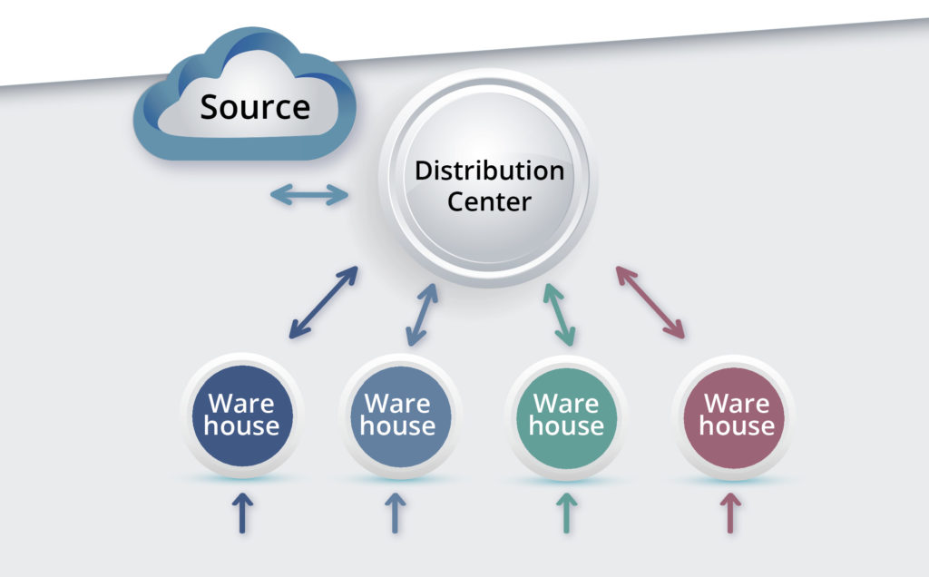
Figure 1: General structure of one type of two-level inventory system

Stay Tuned for our next Blog

COMING SOON. To see an example of a simulation of the system in Figure 1, read the second blog on this topic