
The Smart Forecaster

Consider the problem of replenishing inventory. To be specific, suppose the inventory item in question is a spare part. Both you and your supplier will want some sense of how much you will be ordering and when. And your ERP system may be insisting that you let it in on the secret too.
Deterministic Model of Replenishment
The simplest way to get a decent answer to this question is to assume the world is, well, simple. In this case, simple means “not random” or, in geek speak, “deterministic.” In particular, you pretend that the random size and timing of demand is really a continuous drip-drip-drip of a fixed size coming at a fixed interval, e.g., 2, 2, 2, 2, 2, 2… If this seems unrealistic, it is. Real demand might look more like this: 0, 1, 10, 0, 1, 0, 0, 0 with lots of zeros, occasional but random spikes.
But simplicity has its virtues. If you pretend that the average demand occurs every day like clockwork, it is easy to work out when you will need to place your next order, and how many units you will need. For instance, suppose your inventory policy is of the (Q,R) type, where Q is a fixed order quantity and R is a fixed reorder point. When stock drops to or below the reorder point R, you order Q units more. To round out the fantasy, assume that the replenishment lead time is also fixed: after L days, those Q new units will be on the shelf ready to satisfy demand.
All you need now to answer your questions is the average demand per day D for the item. The logic goes like this:
- You start each replenishment cycle with Q units on hand.
- You deplete that stock by D units per day.
- So, you hit the reorder point R after (Q-R)/D days.
- So, you order every (Q-R)/D days.
- Each replenishment cycle lasts (Q-R)/D + L days, so you make a total of 365D/(Q-R+LD) orders per year.
- As long as lead time L < R/D, you will never stock out and your inventory will be as small as possible.
Figure 1 shows the plot of on-hand inventory vs time for the deterministic model. Around Smart Software, we refer to this plot as the “Deterministic Sawtooth.” The stock starts at the level of the last order quantity Q. After steadily decreasing over the drop time (Q-R)/D, the level hits the reorder point R and triggers an order for another Q units. Over the lead time L, the stock drops to exactly zero, then the reorder magically arrives and the next cycle begins.
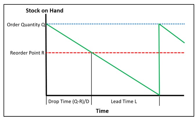
Figure 1: Deterministic model of on-hand inventory
This model has two things going for it. It requires no more than high school algebra, and it combines (almost) all the relevant factors to answer the two related questions: When will we have to place the next order? How many orders will we place in a year?
Probabilistic Model of Replenishment
Not surprisingly, if we strip away some of the fantasy from the deterministic model, we get more useful information. The probabilistic model incorporates all the messy randomness in the real-world problem: the uncertainty in both the timing and size of demand, the variation in replenishment lead time, and the consequences of those two factors: the chance of stock on hand undershooting the reorder point, the chance that there will be a stockout, the variability in the time until the next order, and the variable number of orders executed in a year.
The probabilistic model works by simulating the consequences of uncertain demand and variable lead time. By analyzing the item’s historical demand patterns (and excluding any observations that were recorded during a time when demand may have been fundamentally different), advanced statistical methods create an unlimited number of realistic demand scenarios. Similar analysis is applied to records of supplier lead times. Combining these supply and demand scenarios with the operational rules of any given inventory control policy produces scenarios of the number of parts on hand. From these scenarios, we can extract summaries of the varying intervals between orders.
Figure 2 shows an example of a probabilistic scenario; demand is random, and the item is managed using reorder point R = 10 and order quantity Q=20. Gone is the Deterministic Sawtooth; in its place is something more complex and realistic (the Probabilistic Staircase). During the 90 simulated days of operation, there were 9 orders placed, and the time between orders clearly varied.
Using the probabilistic model, the answers to the two questions (how long between orders and how many in a year) get expressed as probability distributions reflecting the relative likelihoods of various scenarios. Figure 3 shows the distribution of the number of days between orders after ten years of simulated operation. While the average is about 8 days, the actual number varies widely, from 2 to 17.
Instead of telling your supplier that you will place X orders next year, you can now project X ± Y orders, and your supplier knows better their upside and downside risks. Better yet, you could provide the entire distribution as the richest possible answer.
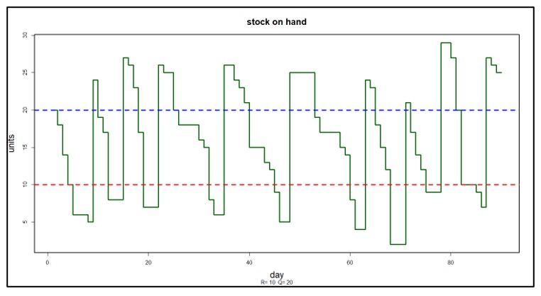
Figure 2 A probabilistic scenario of on-hand inventory
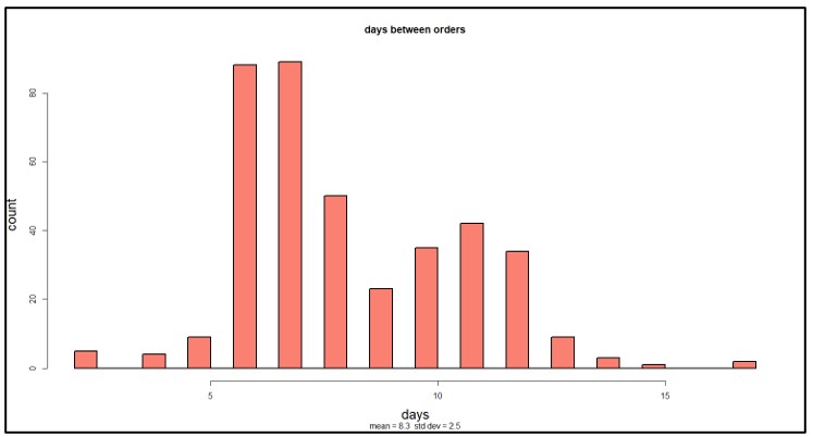
Figure 3: Distribution of days between orders
Climbing the Random Staircase to Greater Efficiency
Moving beyond the deterministic model of inventory opens up new possibilities for optimizing operations. First, the probabilistic model allows realistic assessment of stockout risk. The simple model in Figure 1 implies there is never a stockout, whereas probabilistic scenarios allow for the possibility (though in Figure 2 there was only one close call around day 70). Once the risk is known, software can optimize by searching the “design space” (i.e., all possible values of R and Q) to find a design that meets a target level of stockout risk at minimal cost. The value of the deterministic model in this more realistic analysis is that it provides a good starting point for the search through design space.
Summary
Modern software provides answers to operational questions with various degrees of detail. Using the example of the time between replenishment orders, we’ve shown that the answer can be calculated approximately but quickly by a simple deterministic model. But it can also be provided in much richer detail with all the variability exposed by a probabilistic model. We think of these alternatives as complementary. The deterministic model bundles all the key variables into an easy-to-understand form. The probabilistic model provides additional realism that professionals expect and supports effective search for optimal choices of reorder point and order quantity.


Forecast-Based Inventory Management for Better Planning
Forecast-based inventory management, or MRP (Material Requirements Planning) logic, is a forward-planning method that helps businesses meet demand without overstocking or understocking. By anticipating demand and adjusting inventory levels, it maintains a balance between meeting customer needs and minimizing excess inventory costs. This approach optimizes operations, reduces waste, and enhances customer satisfaction.
Make AI-Driven Inventory Optimization an Ally for Your Organization
In this blog, we will explore how organizations can achieve exceptional efficiency and accuracy with AI-driven inventory optimization. Traditional inventory management methods often fall short due to their reactive nature and reliance on manual processes. Maintaining optimal inventory levels is fundamental for meeting customer demand while minimizing costs. The introduction of AI-driven inventory optimization can significantly reduce the burden of manual processes, providing relief to supply chain managers from tedious tasks.

The Importance of Clear Service Level Definitions in Inventory Management
Inventory optimization software that supports what-if analysis will expose the tradeoff of stockouts vs. excess costs of varying service level targets. But first it is important to identify how “service levels” is interpreted, measured, and reported. This will avoid miscommunication and the false sense of security that can develop when less stringent definitions are used. Clearly defining how service level is calculated puts all stakeholders on the same page. This facilitates better decision-making.