Forecasting inventory requirements is a specialized variant of forecasting that focuses on the high end of the range of possible future demand.

For simplicity, consider the problem of forecasting inventory requirements for just one period ahead, say one day ahead. Usually, the forecasting job is to estimate the most likely or average level of product demand. However, if available inventory equals the average demand, there is about a 50% chance that demand will exceed inventory and result in lost sales and/or lost good will. Setting the inventory level at, say, ten times the average demand will probably eliminate the problem of stockouts, but will just as surely result in bloated inventory costs.

The trick of inventory optimization is to find a satisfactory balance between having enough inventory to meet most demand without tying up too many resources in the process. Usually, the solution is a blend of business judgment and statistics. The judgmental part is to define an acceptable inventory service level, such as meeting 95% of demand immediately from stock. The statistical part is to estimate the 95th percentile of demand.

When not dealing with intermittent demand, you can often estimate the required inventory level by assuming a bell-shaped (Normal) curve of demand, estimating both the middle and the width of the bell curve, then using a standard statistical formula to estimate the desired percentile. The difference between the desired inventory level and the average level of demand is called the “safety stock” because it protects against the possibility of stockouts.

When dealing with intermittent demand, the bell-shaped curve is a very poor approximation to the statistical distribution of demand. In this special case, Smart leverages patented technology for intermittent demand that is designed to accurately forecast the ranges and produce a better estimate of the safety stock needed to achieve the required inventory service level.

Customers often ask us why a stocking recommendation is “so high.” Here is a question we received recently:

During our last team meeting, we found a few items with abnormal gaps between our current ROP and the Smart-suggested ROP at a 99% service level. The concern is that the system indicates that the reorder point will have to increase substantially to achieve a 99% service level. Would you please help us understand the calculation?

When we reviewed the data, it was clear to the customer that the Smart-calculated ROP was indeed correct.  We concluded (1) what they really wanted was a much lower service level target and (2) we had not done a good explaining what was really meant by “service level.” 

So, what does a “99% service level” really mean? 

When it pertains to the target that you enter in your inventory optimization software, it means that the stocking level for the item in question will have a 99% chance of being able to fill whatever the customer needs right away.  For instance, if you have 50 units in stock, there is a 99% chance that the next demand will fall somewhere in the range of 0 to 50 units.

What our customer meant was that 99% of the time a customer placed an order, it was delivered in full within whatever lead time the customer was quoted.  In other words, not necessarily right away but when promised.  

Obviously, the more time you give yourself to deliver to a customer the higher your service level will be. But that distinction is often not explicitly understood when new users of inventory optimization software are conducting what-if scenarios at different service levels.  And that can lead to considerable confusion.  Computing service levels based on immediate stock availability is a higher standard: harder to meet but much more competitive.

Our manufacturing customers often quote service levels based on lead times to their customers, so it isn’t essential for them to deliver immediately from the shelf. In contrast, our customers in the distribution, Maintenance Repair and Operations (MRO), and spare parts spaces, must normally ship same day or within 24 hours.  For them it is a competitive necessity to ship right away and do so in full.

When inputting target service levels using your inventory optimization software, keep this distinction in mind.  Choose the service level based on the percentage of the time you want to ship inventory in full, right away from the shelf.  

Automatic forecasting is the most popular and most used feature of SmartForecasts and Smart Demand Planner. Creating Automatic forecasts is easy. But, the simplicity of Automatic Forecasting masks a powerful interaction of a number of highly effective methods of forecasting. In this blog, we discuss some of the theory behind this core feature. We focus on Automatic forecasting, in part because of its popularity and in part because many other forecasting methods produce similar outputs. Knowledge of Automatic forecasting immediately carries over to Simple Moving Average, Linear Moving Average, Single Exponential Smoothing, Double Exponential Smoothing, Winters’ Exponential Smoothing, and Promo forecasting.

Forecasting tournament

Automatic forecasting works by conducting a tournament among a set of competing methods. Because personal computers and cloud computing are fast, and because we have coded very efficient algorithms into the SmartForecasts’ Automatic forecasting engine, it is practical to take a purely empirical approach to deciding which extrapolative forecasting method to use. This means that you can afford to try out a number of approaches and then retain the one that does best at forecasting the particular data series at hand. SmartForecasts fully automates this process for you by trying the different forecasting methods in a simulated forecasting tournament. The winner of the tournament is the method that comes closest to  predicting new data values from old. Accuracy is measured by average absolute error (that is, the average error, ignoring any minus signs). The average is computed over a set of forecasts, each using a portion of the data, in a process known as sliding simulation.

Sliding simulation

The sliding simulation sweeps repeatedly through ever-longer portions of the historical data, in each case forecasting ahead the desired number of periods in your forecast horizon. Suppose there are 36 historical data values and you need to forecast six periods ahead. Imagine that you want to assess the forecast accuracy of some particular method, say a moving average of four observations, on the data series at hand.

At one point in the sliding simulation, the first 24 points (only) are used to forecast the 25th through 30th historical data values, which we temporarily regard as unknown. We say that points 25-30 are “held out” of the analysis. Computing the absolute values of the differences between the six forecasts and the corresponding actual historical values provides one instance each of a 1-step, 2-step, 3-step, 4-step, 5-step, and 6-step ahead absolute forecast error. Repeating this process using the first 25 points provides more instances of 1-step, 2-step, 3-step ahead errors, and so on. The average over all of the absolute error estimates obtained this way provides a single-number summary of accuracy.

Methods used in Automatic forecasting

Normally, there are six extrapolative forecasting methods competing in the Automatic forecasting tournament:

• Simple moving average
• Linear moving average
• Single exponential smoothing
• Double exponential smoothing
• Additive version of Winters’ exponential smoothing
• Multiplicative version of Winters’ exponential smoothing

The latter two methods are appropriate for seasonal series; however, they are automatically excluded from the tournament if there are fewer than two full seasonal cycles of data (for example, fewer than 24 periods of monthly data or eight periods of quarterly data).

These six classical, smoothing-based methods have proven themselves to be easy to understand, easy to compute and accurate. You can exclude any of these methods from the tournament if you have a preference for some of the competitors and not others.

Lead time delays and supply variability are supply chain facts of life, yet inventory-carrying organizations are often caught by surprise when a supplier is late. An effective inventory planning process embraces this fact of life and develops policies that effectively account for this uncertainty. Sure, there will be times when lead time delays come out of nowhere and cause a shortage. But most often, the shortages result from:

1. Not computing stocking policies (e.g., reorder points, safety stocks, and Min/Max levels) often enough to catch changes in the lead time. 
2. Using poor estimates of actual lead time such as using only averages of historical receipts or relying on a supplier quote.

Instead, recalibrate policies across every single part during every planning cycle to catch changes in demand and lead times.  Rather than assuming only an average lead time, simulate the lead times using scenarios.  This way, recommended stocking policies account for the probabilities of lead times being high and adjust accordingly.  When you do this, you’ll identify needed inventory increases before it is too late. You’ll capture more sales and drive significant improvements in customer satisfaction.

Is safety stock regarded as emergency spares or as a day-to-day buffer against spikes in demand? Knowing the difference and configuring your ERP properly will make a big difference to your bottom line.

The Safety Stock field in your ERP system can mean very different things depending on the configuration. Not understanding these differences and how they impact your bottom line is a common issue we’ve seen arise in implementations of our software.

Implementing inventory optimization software starts with new customers completing the technical implementation to get data flowing.  They then receive user training and spend weeks carefully configuring their initial safety stocks, reorder levels, and consensus demand forecasts with Smart IP&O.  The team becomes comfortable with Smart’s key performance predictions (KPPs) for service levels, ordering costs, and inventory on hand, all of which are forecasted using the new stocking policies.

But when they save the policies and forecasts to their ERP test system, sometimes the orders being suggested are far larger and more frequent than they expected, driving up projected inventory costs.

When this happens, the primary culprit is how the ERP is configured to treat safety stock.  Being aware of these configuration settings will help planning teams better set expectations and achieve the expected outcomes with less effort (and cause for alarm!).

Here are the three common examples of ERP safety stock configurations:

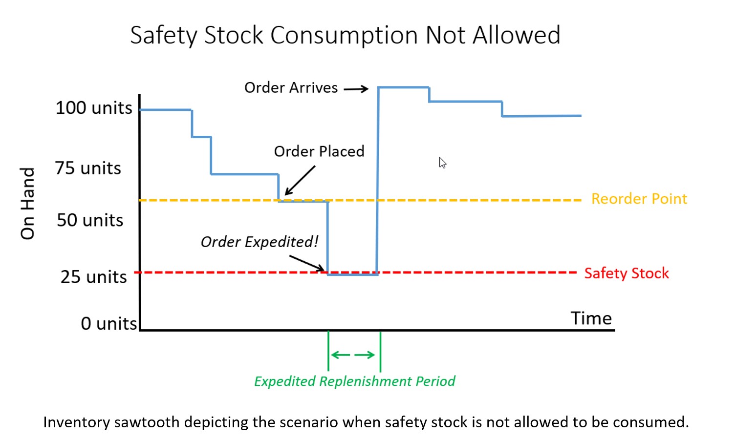
Configuration 1. Safety Stock is treated as emergency stock that can’t be consumed. If a breach of safety stock is predicted, the ERP system will force an expedite no matter the cost so the inventory on hand never falls below safety stock, even if a scheduled receipt is already on order and scheduled to arrive soon.

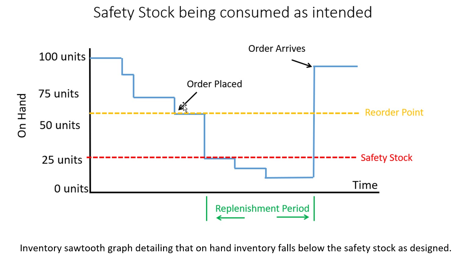
Configuration 2. Safety Stock is treated as Buffer stock that is designed to be consumed. The ERP system will place an order when a breach of safety stock is predicted but on hand inventory will be allowed to fall below the safety stock. The buffer stock protects against stockout during the resupply period (i.e., the lead time).

Configuration 3. Safety Stock is ignored by the system and treated as a visual planning aid or rule of thumb. It is ignored by supply planning calculations but used by the planner to help make manual assessments of when to order.

Note: We never recommend using the safety stock field as described in Configuration 3. In most cases, these configurations were not intended but result from years of improvisation that have led to using the ERP in a non-standard way.  Generally, these fields were designed to programmatically influence the replenishment calculations.  So, the focus of our conversation will be on Configurations 1 and 2. 

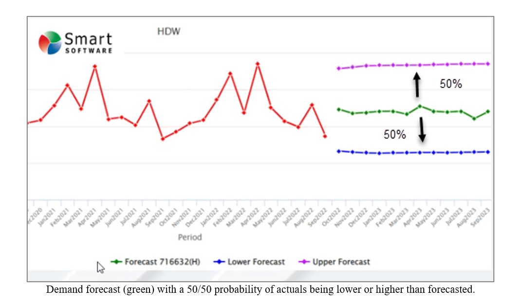
Forecasting and inventory optimization systems are designed to compute forecasts that will anticipate inventory draw down and then calculate safety stocks sufficient to protect against variability in demand and supply. This means that the safety stock is intended to be used as a protective buffer (Configuration 2) and not as emergency sparse (Configuration 3).  It is also important to understand that, by design, the safety stock will be consumed approximately 50% of the time.

Why 50%? Because actual orders will exceed an unbiased forecast half of the time. See the graphic below illustrating this.  A “good” forecast should yield the value that will come closest to the actual most often so actual demand will either be higher or lower without bias in either direction.

If you configured your ERP system to properly allow consumption of safety stock, then the on hand inventory might look like the graph below.  Note that some safety stock is consumed but avoided a stockout.  The service level you target when computing safety stock will dictate how often you stockout before the replenishment order arrives.  Average inventory is roughly 60 units over the time horizon in this scenario.

If your ERP system is configured to not allow consumption of safety stock and treats the quantity entered in the safety stock field more like emergency spares, then you will have a massive overstock!  Your inventory on hand would look like the graph below with orders being expedited as soon as a breach of safety stock is expected. Average inventory is roughly 90 units, a 50% increase compared to when you allowed safety stock to be consumed.