If you keep up with the news about supply chain analytics, you are more frequently encountering the phrase “probabilistic forecasting.” If this phrase is puzzling, read on.
You probably already know what “forecasting” means. And you probably also know that there seem to be lots of different ways to do it. And you’ve probably heard pungent little phrases like “every forecast is wrong.” So you know that some kind of mathemagic might calculate that “the forecast is you will sell 100 units next month”, and then you might sell 110 units, in which case you have a 10% forecast error.
You may not know that what I just described is a particular kind of forecast called a “point forecast.” A point forecast is so named because it consists of just a single number (i.e., one point on the number line, if you recall the number line from your youth).
Point forecasts have one virtue: They are simple. They also have a flaw: They give rise to snarky statements like “every forecast is wrong.” That is, in most realistic cases, it is unlikely that the actual value will exactly equal the forecast. (Which isn’t such a big deal if the forecast is close enough.)
This gets us to “probabilistic forecasting.” This approach is a step up, because instead of producing a single-number (point) forecast, it yields a probability distribution for the forecast. And unlike traditional extrapolative models that rely purely on the historical data, probabilistic forecasts have the ability to simulate future values that aren’t anchored to the past.
“Probability distribution” is a forbidding phrase, evoking some arcane math that you may have heard of but never studied. Luckily, most adults have enough life experience to have an intuitive grasp of the concept. When broken down, it’s quite straightforward to understand.
Imagine the simple act of flipping two coins. You might call this harmless fun, but I call it a “probabilistic experiment.” The total number of heads that turn up on the two coins will be either zero, one or two. Flipping two coins is a “random experiment.” The resulting number of heads is a “random variable.” It has a “probability distribution”, which is nothing more than a table of how likely it is that the random variable will turn out to have any of its possible values. The probability of getting two heads when the coins are fair works out to be ¼, as is the probability of no heads. The chance of one head is ½.
The same approach can describe a more interesting random variable, like the daily demand for a spare part. Figure 2 shows such a probability distribution. It was computed by compiling three years of daily demand data on a certain part used in a scientific instrument sold to hospitals.

Figure 1: The probability distribution of daily demand for a certain spare part
The distribution in Figure 1 can be thought of as a probabilistic forecast of demand in a single day. For this particular part, we see that the forecast is very likely to be zero (97% chance), but sometimes will be for a handful of units, and once in three years will be twenty units. Even though the most likely forecast is zero, you would want to keep a few on hand if this part were critical (“…for want of a nail…”)
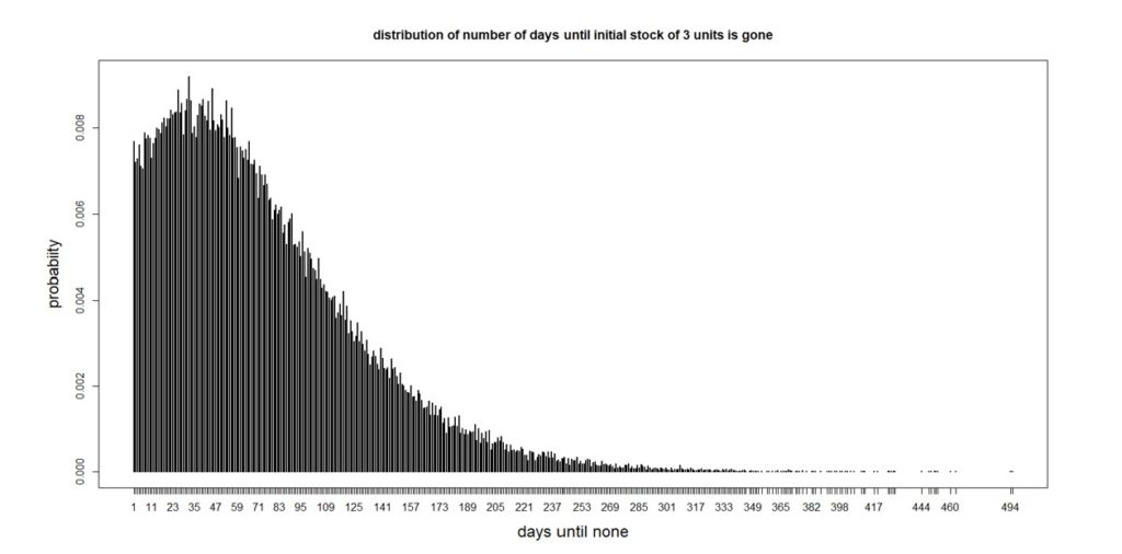
Now let’s use this information to make a more complicated probabilistic forecast. Suppose you have three units on hand. How many days will it take for you to have none? There are many possible answers, ranging from a single day (if you immediately get a demand for three or more) up to a very large number (since 97% of days see no demand). The analysis of this question is a bit complicated because of all the many ways this situation can play out, but the final answer that is most informative will be a probability distribution. It turns out that the number of days until there are no units left in stock has the distribution shown in Figure 2.

Figure 2: Distribution of the number of days until all three units are gone
The average number of days is 74, which would be a point forecast, but there is a lot of variation around the average. From the perspective of inventory management, it is notable that there is a 25% chance that all the units will be gone after 32 days. So if you decided to order more when you were down to only three on the shelf, it would be good to have the supplier get them to you before a month has passed. If they couldn’t, you’d have a 75% chance of stocking out – not good for a critical part.
The analysis behind Figure 2 involved making some assumptions that were convenient but not necessary if they were not true. The results came from a method called “Monte Carlo simulation”, in which we start with three units, pick a random demand from the distribution in Figure 1, subtract it from the current stock, and continue until the stock is gone, recording how many days went by before you ran out. Repeating this process 100,000 times produced Figure 2.
Applications of Monte Carlo simulation extend to problems of even larger scope than the “when do we run out” example above. Especially important are Monte Carlo forecasts of future demand. While the usual forecasting result is a set of point forecasts (e.g., expected unit demand over the next twelve months), we know that there are any number of ways that the actual demand could play out. Simulation could be used to produce, say, one thousand possible sets of 365 daily demand demands.
This set of demand scenarios would more fully expose the range of possible situations with which an inventory system would have to cope. This use of simulation is called “stress testing”, because it exposes a system to a range of varied but realistic scenarios, including some nasty ones. Those scenarios are then input to mathematical models of the system to see how well it will cope, as reflected in key performance indicators (KPI’s). For instance, in those thousand simulated years of operation, how many stockouts are there in the worst year? the average year? the best year? In fact, what is the full probability distribution of the number of stockouts in a year, and what is the distribution of their size?
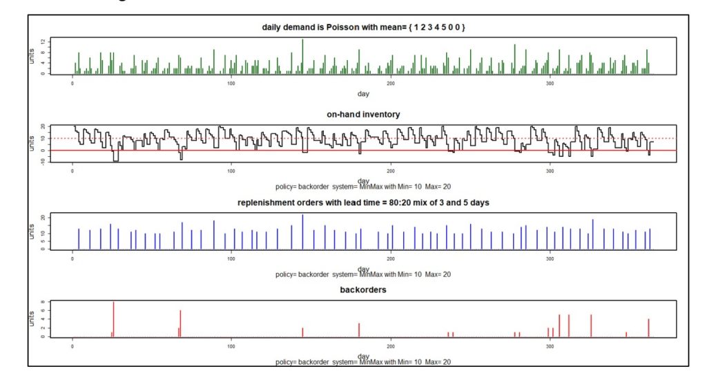
Figures 3 and 4 illustrate probabilistic modeling of an inventory control system that converts stockouts to backorders. The system simulated uses a Min/Max control policy with Min = 10 units and Max = 20 units.
Figure 3 shows one simulated year of daily operations in four plots. The first plot shows a particular pattern of random daily demand in which average demand increases steadily from Monday to Friday but disappears on weekends. The second plot shows the number of units on hand each day. Note that there are a dozen times during this simulated year when inventory goes negative, indicating stockouts. The third plot shows the size and timing of replenishment orders. The fourth plot shows the size and timing of backorders. The information in these plots can be translated into estimates of inventory investment, average units on hand, holding costs, ordering costs and shortage costs.

Figure 3: One simulated year of inventory system operation
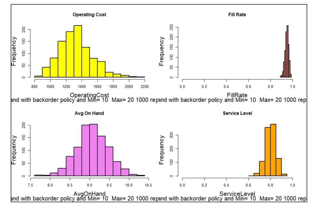
Figure 3 shows one of one thousand simulated years. Each year will have different daily demands, resulting in different values of metrics like units on hand and the various components of operating cost. Figure 4 plots the distribution of 1,000 simulated values of four KPI’s. Simulating 1,000 years of imagined operation exposes the range of possible results so that planners can account not just for average results but also see best-case and worst-case values.

Figure 4: Distributions of four KPI’s based on 1,000 simulations
Monte Carlo simulation is a low-math/high-results approach to probabilistic forecasting: very practical and easy to explain. Advanced probabilistic forecasting methods employed by Smart Software expand upon standard Monte Carlo simulation, yielding extremely accurate estimates of required inventory levels.
Related Posts

Make AI-Driven Inventory Optimization an Ally for Your Organization
In this blog, we will explore how organizations can achieve exceptional efficiency and accuracy with AI-driven inventory optimization. Traditional inventory management methods often fall short due to their reactive nature and reliance on manual processes. Maintaining optimal inventory levels is fundamental for meeting customer demand while minimizing costs. The introduction of AI-driven inventory optimization can significantly reduce the burden of manual processes, providing relief to supply chain managers from tedious tasks.

Daily Demand Scenarios
In this Videoblog, we will explain how time series forecasting has emerged as a pivotal tool, particularly at the daily level, which Smart Software has been pioneering since its inception over forty years ago. The evolution of business practices from annual to more refined temporal increments like monthly and now daily data analysis illustrates a significant shift in operational strategies.

Constructive Play with Digital Twins
Those of you who track hot topics will be familiar with the term “digital twin.” Those who have been too busy with work may want to read on and catch up. While there are several definitions of digital twin, here’s one that works well: A digital twin is a dynamic virtual copy of a physical asset, process, system, or environment that looks like and behaves identically to its real-world counterpart. A digital twin ingests data and replicates processes so you can predict possible performance outcomes and issues that the real-world product might undergo.


