You Need to Team up with the Algorithms

Over forty years ago, Smart Software consisted of three friends working to start a company in a church basement. Today, our team has expanded to operate from multiple locations across Massachusetts, New Hampshire and Texas, with team members in England, Spain, Armenia and India. Like many of you in your jobs,  we have found ways to make distributed teams work for us and for you.

This note is about a different kind of teamwork: the collaboration between you and our software that happens at your fingertips. I often write about the software itself and what goes on “under the hood”. This time, my subject is how you should best team up with the software.

Our software suite, Smart Inventory Planning and Optimization (Smart IP&O™) is capable of massively detailed calculations of future demand and the inventory control parameters (e.g., reorder points and order quantities) that would most effectively manage that demand. But your input is required to make the most of all that power. You need to team up with the algorithms.

That interaction can take several forms. You can start by simply assessing how you are doing now. The report writing functions in Smart IP&O (Smart Operational Analytics™) can collate and analyze all your transactional data to measure your Key Performance Indicators (KPIs), both financial (e.g., inventory investment) and operational (e.g., fill rates).

The next step might be to use SIO (Smart Inventory Optimization™), the inventory analytics within SIP&O, to play “what-if” games with the software. For example, you might ask “What if we reduced the order quantity on item 1234 from 50 to 40?” The software grinds the numbers to let you know how that would play out, then you react. This can be useful, but what if you have 50,000 items to consider? You would want to do what-if games for a few critical items, but not all of them.

The real power comes with using the automatic optimization capability in SIO. Here you can team with the algorithms at scale. Using your business judgement, you can create “groups”, i.e., collections of items that share some critical features. For example, you might create a group for “critical spare parts for electric utility customers” consisting of 1,200 parts. Then again calling on your business judgement, you could specify what item availability standard should apply to all the items in that group (e.g., “at least 95% chance of not stocking out in a year”). Now the software can take over and automatically work out the best reorder points and order quantities for every one of those items to achieve your required item availability at the lowest possible total cost. And that, dear reader, is powerful teamwork.


How Are We Doing? KPI’s and KPP’s

Dealing with the day-to-day of inventory management can keep you busy. There’s the usual rhythm of ordering, receiving, forecasting and planning, and moving things around in the warehouse. Then there are the frenetic times – shortages, expedites, last-minute calls to find new suppliers.

All this activity works against taking a moment to see how you’re doing. But you know you have to get your head up now and then to see where you’re heading. For that, your inventory software should show you metrics – and not just one, but a full set of metrics or KPI’s – Key Performance Indicators.

Multiple Metrics

Depending on your role in your organization, different metrics will have different salience. If you are on the finance side of the house, inventory investment may be top of mind: how much cash is tied up in inventory? If you’re on the sales side, item availability may be top of mind: what’s the chance that I can say “yes” to an order? If you’re responsible for replenishment, how many PO’s will your people have to cut in the next quarter?

Availability Metrics

Let’s circle back to item availability. How do you put a number on that? The two most used availability metrics are “service level” and “fill rate.” What’s the difference? It’s the difference between saying “We had an earthquake yesterday” and saying, “We had an earthquake yesterday, and it was a 6.4 on the Richter scale.” Service level records the frequency of stockouts no matter their size; fill rate reflects their severity. The two can seem to point in opposite directions, which causes some confusion. You can have a good service level, say 90%, but have an embarrassing fill rate, say 50%. Or vice versa. What makes them different is the distribution of demand sizes. For instance, if the distribution is very skewed, so most demands are small but some are huge, you might get the 90%/50% split mentioned above. If your focus is on how often you have to backorder, service level is more relevant. If your worry is how big an overnight expedite can get, the fill rate is more relevant.

One Graph to Rule them All

A graph of on-hand inventory can provide the basis for calculating multiple KPI’s. Consider Figure 1, which plots on-hand each day for a year. This plot has information needed to calculate multiple metrics: inventory investment, service level, fill rate, reorder rate and other metrics.

Key performace indicators and paramenters for inventory management

Inventory investment: The average height of the graph when above zero, when multiplied by unit cost of the inventory item, gives quarterly dollar value.

Service level: The fraction of inventory cycles that end above zero is the service level. Inventory cycles are marked by the up movements occasioned by the arrival of replenishment orders.

Fill rate: The amount by which inventory drops below zero and how long it stays there combine to determine fill rate.

In this case, the average number of units on hand was 10.74, the service level was 54%, and the fill rate was 91%.


KPI’s and KPP’s

In the over forty years since we founded Smart Software, I have never seen a customer produce a plot like Figure 1.  Those who are further along in their development do produce and pay attention to reports listing their KPI’s in tabular form, but they don’t look at such a graph. Nevertheless, that graph has value for developing insight into the random rhythms of inventory as it rises and falls.

Where it is especially useful is prospectively. Given market volatility, key variables like supplier lead times, average demand, and demand variability all shift over time. This implies that key control parameters like reorder points and order quantities must adjust to these shifts. For instance, if a supplier says they’ll have to increase their average lead time by 2 days, this will impact your metrics negatively, and you may need to increase your reorder point to compensate. But increase it by how much?

Here is where modern inventory software comes in. It will let you propose an adjustment and then see how things will play out. Plots like Figure 1 let you see and get a feel for the new regime. And the plots can be analyzed to compute KPP’s – Key Performance Predictions.

KPP’s help take the guesswork out of adjustments. You can simulate what will happen to your KPI’s if you change them in response to changes in your operating environment – and how bad things will get if you make no changes.


Confused about AI and Machine Learning?

Are you confused about what is AI and what is machine learning? Are you unsure why knowing more will help you with your job in inventory planning? Don’t despair. You’ll be ok, and we’ll show you how some of whatever-it-is can be useful.

What is and what isn’t

What is AI and how does it differ from ML? Well, what does anybody do these days when they want to know something? They Google it. And when they do, the confusion starts.

One source says that the neural net methodology called deep learning is a subset of machine learning, which is a subset of AI. But another source says that deep learning is already a part of AI because it sort of mimics the way the human mind works, while machine learning doesn’t try to do that.

One source says there are two types of machine learning: supervised and unsupervised. Another says there are four: supervised, unsupervised, semi-supervised and reinforcement.

Some say reinforcement learning is machine learning; others call it AI.

Some of us traditionalists call a lot of it “statistics”, though not all of it is.

In the naming of methods, there is a lot of room for both emotion and salesmanship. If a software vendor thinks you want to hear the phrase “AI”, they may well say it for you just to make you happy.

Better to focus on what comes out at the end

You can avoid some confusing hype if you focus on the end result you get from some analytic technology, regardless of its label. There are several analytical tasks that are relevant to inventory planners and demand planners. These include clustering, anomaly detection, regime change detection, and regression analysis. All four methods are usually, but not always, classified as machine learning methods. But their algorithms can come straight out of classical statistics.

Clustering

Clustering means grouping together things that are similar and distancing them from things that are dissimilar. Sometimes clustering is easy: to separate your customers geographically, simply sort them by state or sales region. When the problem is not so dead obvious, you can use data and clustering algorithms to get the job done automatically even when dealing with massive datasets.

For example, Figure 1 illustrates a cluster of “demand profiles”, which in this case divides all a customer’s items into nine clusters based on the shape of their cumulative demand curves. Cluster 1.1 in the top left contains items whose demand has been petering out, while Cluster 3.1 in the bottom left contains items whose demand has accelerated.  Clustering can also be done on suppliers. The choice of number of clusters is typically left to user judgement, but ML can guide that choice.  For example, a user might instruct the software to “break my parts into 4 clusters” but using ML may reveal that there are really 6 distinct clusters the user should analyze. 


Confused about AI and Machine Learning Inventory Planning

Figure 1: Clustering items based on the shapes of their cumulative demand

Anomaly Detection

Demand forecasting is traditionally done using time series extrapolation. For instance, simple exponential smoothing works to find the “middle” of the demand distribution at any time and project that level forward. However, if there has been a sudden, one-time jump up or down in demand in the recent past, that anomalous value can have a significant but unwelcome effect on the near-term forecast.  Just as serious for inventory planning, the anomaly can have an outsized effect on the estimate of demand variability, which goes directly to the calculation of safety stock requirements.

Planners may prefer to find and remove such anomalies (and maybe do offline follow-up to find out the reason for the weirdness). But nobody with a big job to do will want to visually scan thousands of demand plots to spot outliers, expunge them from the demand history, then recalculate everything. Human intelligence could do that, but human patience would soon fail. Anomaly detection algorithms could do the work automatically using relatively straightforward statistical methods. You could call this “artificial intelligence” if you wish.

Regime Change Detection

Regime change detection is like the big brother of anomaly detection. Regime change is a sustained, rather than temporary, shift in one or more aspects of the character of a time series. While anomaly detection usually focuses on sudden shifts in mean demand, regime change could involve shifts in other features of the demand, such as its volatility or its distributional shape.  

Figure 2 illustrates an extreme example of regime change. The bottom dropped out of demand for this item around day 120. Inventory control policies and demand forecasts based on the older data would be wildly off base at the end of the demand history.

Confused about AI and Machine Learning Demand Planning

Figure 2: An example of extreme regime change in an item with intermittent demand

Here too, statistical algorithms can be developed to solve this problem, and it would be fair play to call them “machine learning” or “artificial intelligence” if so motivated.  Using ML or AI to identify regime changes in demand history enables demand planning software to automatically use only the relevant history when forecasting instead of having to manually pick the amount of history to introduce to the model. 

Regression analysis

Regression analysis relates one variable to another through an equation. For example, sales of window frames in one month may be predicted from building permits issued a few months earlier. Regression analysis has been considered a part of statistics for over a century, but we can say it is “machine learning” since an algorithm works out the precise way to convert knowledge of one variable into a prediction of the value of another.

Summary

It is reasonable to be interested in what’s going on in the areas of machine learning and artificial intelligence. While the attention given to ChatGPT and its competitors is interesting, it is not relevant to the numerical side of demand planning or inventory management. The numerical aspects of ML and AI are potentially relevant, but you should try to see through the cloud of hype surrounding these methods and focus on what they can do.  If you can get the job done with classical statistical methods, you might just do that, then exercise your option to stick the ML label on anything that moves.


Maximize Machine Uptime with Probabilistic Modeling

The Smart Forecaster

 Pursuing best practices in demand planning,

forecasting and inventory optimization

Two Inventory Problems

If you both make and sell things, you own two inventory problems. Companies that sell things must focus relentlessly on having enough product inventory to meet customer demand.  Manufacturers and asset intensive industries such as power generation, public transportation, mining, and refining, have an additional inventory concern:  having enough spare parts to keep their machines running. This technical brief reviews the basics of two probabilistic models of machine breakdown. It also relates machine uptime to the adequacy of spare parts inventory.


Modeling the failure of a machine treated as a “black box”

Just as product demand is inherently random, so is the timing of machine breakdowns. Likewise, just as probabilistic modeling is the right way to deal with random demand, it is also the right way to deal with random breakdowns.

Models of machine breakdown have two components. The first deals with the random duration of uptime. The second deals with the random duration of downtime.

The field of reliability theory offers several standard probability models describing the random time until failure of a machine without regard for the reason for the failure. The simplest model of uptime is the exponential distribution. This model says that the hazard rate, i.e., the chance of failing in the next instant of time, is constant no matter how long the system has been operating. The exponential model does a good job at modeling certain types of systems, especially electronics, but it is not universally applicable.


Download the Whitepaper


The next step up in model complexity is the Weibull model (pronounced “WHY-bull”). The Weibull distribution allows the risk of failure to change over time, either decreasing after a burn in period or, more often, increasing as wear and tear accumulate. The exponential distribution is a special case of the Weibull distribution in which the hazard rate is neither increasing nor decreasing.

Weibull Reliability Plot

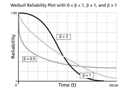
Figure 1: Three different Weibull survival curves

Figure 1 illustrates the Weibull model’s probability that a machine is still running as a function of how long it has been running. There are three curves corresponding to constant, decreasing and increasing hazard rates. For obvious reasons, these are called survival curves because they plot the probability of surviving for various amounts of time (but they are also called reliability curves). The black curve that starts high and sinks fast (β=3) depicts a machine that wears out with age. The lightest curve in the middle fast (β=1) shows the exponential distribution. The medium-dark curve (β=0.5)  is one that has a high early hazard rate but gets better with age.

Of course, there is another phenomenon that needs to be included in the analysis: downtime. Modeling downtime is where inventory theory enters the picture. Downtime is modeled by a mixture of two different distributions. If a spare part is available to replace the failed part, then the downtime can be very brief, say one day. But if there is no spare in stock, then the downtime can be quite long. Even if the spare can be obtained on an expedited basis, it may be several days or a week before the machine can be repaired. If the spare must be fabricated by a far-away supplier and shipped by sea then by rail then trucked to your plant, the downtime could be weeks or months. This all means that keeping a proper inventory of spares is very important to keeping production humming along.

In this aggregated type of analysis, the machine is treated as a black box that is either working or not. Though ignoring the details of which part failed and when, such a model is useful for sizing the pool of machines needed to maintain some minimum level of production capacity with high probability.

The binomial distribution is the probability model relevant to this problem. The binomial is the same model that describes, for example, the distribution of the number of “heads” resulting from twenty tosses of a coin. In the machine reliability problem, the machines correspond to coins, and an outcome of heads corresponds to having a working machine.

As an example, if

  • the chance that any given machine is running on any particular day is 90%
  • machine failures are independent (e.g., no flood or tornado to wipe them all out at once)
  • you require at least a 95% chance that at least 5 machines are running on any given day

then the binomial model prescribes seven machines to achieve your goal.


Modeling machine failures based on component failures

Maximize Machine Uptime with Probabilistic Modeling

The Weibull model can also be used to describe the failure of a single part. However, any realistically complex production machine will have multiple parts and therefore have multiple failure modes. This means that calculating the time until the machine fails requires analysis of a “race to failure”, with each part vying for the “honor” of being the first to fail.

If we make the reasonable assumption that parts fail independently, standard probability theory points the way to combining the models of individual part failure into an overall model of machine failure. The time until the first of many parts fails has a poly-Weibull distribution. At this point, though, the analysis can get quite complicated, and the best move may be to switch from analysis-by-equation to analysis-by-simulation.


Simulating machine failure from the details of part failures

Simulation analysis got its modern start as a spinoff of the Manhattan Project to build the first atomic bomb. The method is also commonly called Monte Carlo simulation after the biggest gambling center on earth back in the day (today it would be “Macau simulation”).

A simulation model converts the logic of the sequence of random events into corresponding computer code. Then it uses computer-generated (pseudo-)random numbers as fuel to drive the simulation model. For example, each component’s failure time is created by drawing from its particular Weibull failure time distribution. Then the soonest of those failure times begins the next episode of machine downtime.

simulation of machine uptime over one year of operation

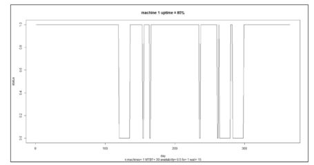
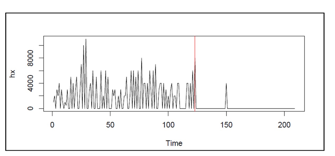
Figure 2: A simulation of machine uptime over one year of operation

Figure 2 shows the results of a simulation of the uptime of a single machine. Machines cycle through alternating periods of uptime and downtime. In this simulation, uptime is assumed to have an exponential distribution with an average duration (MTBF = Mean Time Before Failure) of 30 days. Downtime has a 50:50 split between 1 day if a spare is available and 30 days if not. In the simulation shown in Figure 2, the machine is working during 85% of the days in one year of operation.


An approximate formula for machine uptime

Although Monte Carlo simulation can provide more exact results, a simpler algebraic model does well as an approximation and makes it easier to see how the key variables relate.

Define the following key variables:

  • MTBF = Mean Time Before Failure (days)
  • Pa = Probability that there is a spare part available when needed
  • MDTshort = Mean Down Time if there is a spare available when needed
  • MDTlong = Mean Down Time if there is no spare available when needed
  • Uptime = Percentage of days in which the machine is up and running.

Then there is a simple approximation for the Uptime:

Uptime ≈ 100 x MTBF/(MTBF + MDTshort x Pa + MDTlong x (1-Pa)).    (Equation 1)

Equation 1 tells us that the uptime depends on the availability of a spare. If there is always a spare (Pa=1), then uptime achieves a peak value of about 100 x MTBF/(MTBF + MDTshort). If there is never a spare available (Pa=0), then uptime achieve its lowest value of about 100 x MTBF/(MTBF + MDTlong). When the repair time is about as long as the typical time between failures, uptime sinks to an unacceptable level near 50%. If a spare is always available, uptime can approach 100%.

Relating machine downtime to spare parts inventory

Minimizing downtime requires a multi-pronged initiative involving intensive operator training, use of quality raw materials, effective preventive maintenance – and adequate spare parts. The first three set the conditions for good results. The last deals with contingencies.

Inventory Planning for Manufacturers MRO SAAS

Once a machine is down, money is flying out the door and there is a premium on getting it back up pronto. This scene could play out in two ways. The good one has a spare part ready to go, so the downtime can be kept to a minimum. The bad one has no available spare, so there is a scramble to expedite delivery of the needed part. In this case, the manufacturer must bear both the cost of lost production and the cost of expedited shipping, if that is even an option.

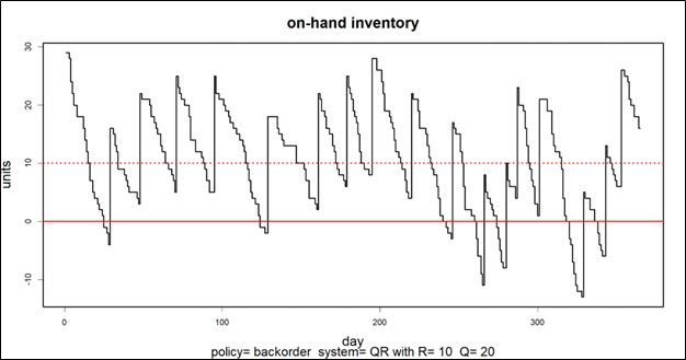
If the inventory system is properly designed, spare parts availability will not be a major impediment to machine uptime. By the design of an inventory system, I mean the results of several choices: whether the shortage policy is a backorder policy or a loss policy, whether the inventory review cycle is periodic or continuous, and what reorder points and order quantities are established.

When inventory policies for products are designed, they are evaluated using several criteria. Service Level is the percentage of replenishment periods that pass without a stockout. Fill Rate is the percentage of units ordered that is supplied immediately from stock. Average Inventory Level is the typical number of units on hand.

None of these is exactly the metric needed for spare parts stocking, though they all are related. The needed metric is Item Availability, which is the percentage of days in which there is at least one spare ready for use. Higher Service Levels, Fill Rates, and Inventory Levels all imply high Item Availability, and there are ways to convert from one to the other. (When dealing with multiple machines sharing the same stock of spares, Inventory Availability gets replaced by the probability distribution of the number of spares on any given day. We leave that more complex problem for another day.)

Clearly, keeping a good supply of spares reduces the costs of machine downtime. Of course, keeping a good supply of spares creates its own inventory holding and ordering costs. This is the manufacturer’s second inventory problem. As with any decision involving inventory, the key is to strike the right balance between these two competing cost centers. See this article on probabilistic forecasting for intermittent demand for guidance on striking that balance.


Leave a Comment

Related Posts

Direct to the Brain of the Boss – Inventory Analytics and Reporting

Direct to the Brain of the Boss – Inventory Analytics and Reporting

In this blog, the spotlight is cast on the software that creates reports for management, the silent hero that translates the beauty of furious calculations into actionable reports. Watch as the calculations, intricately guided by planners utilizing our software, seamlessly converge into Smart Operational Analytics (SOA) reports, dividing five key areas: inventory analysis, inventory performance, inventory trending, supplier performance, and demand anomalies.

How Are We Doing? KPI’s and KPP’s

How Are We Doing? KPI’s and KPP’s

Dealing with the day-to-day of inventory management can keep you busy. But you know you have to get your head up now and then to see where you’re heading. For that, your inventory software should show you metrics – and not just one, but a full set of metrics or KPI’s – Key Performance Indicators.

Confused about AI and Machine Learning?

Confused about AI and Machine Learning?

Are you confused about what is AI and what is machine learning? Are you unsure why knowing more will help you with your job in inventory planning? Don’t despair. You’ll be ok, and we’ll show you how some of whatever-it-is can be useful.

Recent Posts

  • Managing Spare Parts Inventory: Best PracticesManaging Spare Parts Inventory: Best Practices
    In this blog, we’ll explore several effective strategies for managing spare parts inventory, emphasizing the importance of optimizing stock levels, maintaining service levels, and using smart tools to aid in decision-making. Managing spare parts inventory is a critical component for businesses that depend on equipment uptime and service reliability. Unlike regular inventory items, spare parts often have unpredictable demand patterns, making them more challenging to manage effectively. An efficient spare parts inventory management system helps prevent stockouts that can lead to operational downtime and costly delays while also avoiding overstocking that unnecessarily ties up capital and increases holding costs. […]
  • 5 Ways to Improve Supply Chain Decision Speed5 Ways to Improve Supply Chain Decision Speed
    The promise of a digital supply chain has transformed how businesses operate. At its core, it can make rapid, data-driven decisions while ensuring quality and efficiency throughout operations. However, it's not just about having access to more data. Organizations need the right tools and platforms to turn that data into actionable insights. This is where decision-making becomes critical, especially in a landscape where new digital supply chain solutions and AI-driven platforms can support you in streamlining many processes within the decision matrix. […]
  • Two employees checking inventory in temporary storage in a distribution warehouse.12 Causes of Overstocking and Practical Solutions
    Managing inventory effectively is critical for maintaining a healthy balance sheet and ensuring that resources are optimally allocated. Here is an in-depth exploration of the main causes of overstocking, their implications, and possible solutions. […]
  • FAQ Mastering Smart IP&O for Better Inventory ManagementFAQ: Mastering Smart IP&O for Better Inventory Management.
    Effective supply chain and inventory management are essential for achieving operational efficiency and customer satisfaction. This blog provides clear and concise answers to some basic and other common questions from our Smart IP&O customers, offering practical insights to overcome typical challenges and enhance your inventory management practices. Focusing on these key areas, we help you transform complex inventory issues into strategic, manageable actions that reduce costs and improve overall performance with Smart IP&O. […]
  • 7 Key Demand Planning Trends Shaping the Future7 Key Demand Planning Trends Shaping the Future
    Demand planning goes beyond simply forecasting product needs; it's about ensuring your business meets customer demands with precision, efficiency, and cost-effectiveness. Latest demand planning technology addresses key challenges like forecast accuracy, inventory management, and market responsiveness. In this blog, we will introduce critical demand planning trends, including data-driven insights, probabilistic forecasting, consensus planning, predictive analytics, scenario modeling, real-time visibility, and multilevel forecasting. These trends will help you stay ahead of the curve, optimize your supply chain, reduce costs, and enhance customer satisfaction, positioning your business for long-term success. […]

    Inventory Optimization for Manufacturers, Distributors, and MRO

    • Managing Spare Parts Inventory: Best PracticesManaging Spare Parts Inventory: Best Practices
      In this blog, we’ll explore several effective strategies for managing spare parts inventory, emphasizing the importance of optimizing stock levels, maintaining service levels, and using smart tools to aid in decision-making. Managing spare parts inventory is a critical component for businesses that depend on equipment uptime and service reliability. Unlike regular inventory items, spare parts often have unpredictable demand patterns, making them more challenging to manage effectively. An efficient spare parts inventory management system helps prevent stockouts that can lead to operational downtime and costly delays while also avoiding overstocking that unnecessarily ties up capital and increases holding costs. […]
    • Innovating the OEM Aftermarket with AI-Driven Inventory Optimization XLInnovating the OEM Aftermarket with AI-Driven Inventory Optimization
      The aftermarket sector provides OEMs with a decisive advantage by offering a steady revenue stream and fostering customer loyalty through the reliable and timely delivery of service parts. However, managing inventory and forecasting demand in the aftermarket is fraught with challenges, including unpredictable demand patterns, vast product ranges, and the necessity for quick turnarounds. Traditional methods often fall short due to the complexity and variability of demand in the aftermarket. The latest technologies can analyze large datasets to predict future demand more accurately and optimize inventory levels, leading to better service and lower costs. […]
    • Future-Proofing Utilities. Advanced Analytics for Supply Chain OptimizationFuture-Proofing Utilities: Advanced Analytics for Supply Chain Optimization
      Utilities in the electrical, natural gas, urban water, and telecommunications fields are all asset-intensive and reliant on physical infrastructure that must be properly maintained, updated, and upgraded over time. Maximizing asset uptime and the reliability of physical infrastructure demands effective inventory management, spare parts forecasting, and supplier management. A utility that executes these processes effectively will outperform its peers, provide better returns for its investors and higher service levels for its customers, while reducing its environmental impact. […]
    • Centering Act Spare Parts Timing Pricing and ReliabilityCentering Act: Spare Parts Timing, Pricing, and Reliability
      In this article, we'll walk you through the process of crafting a spare parts inventory plan that prioritizes availability metrics such as service levels and fill rates while ensuring cost efficiency. We'll focus on an approach to inventory planning called Service Level-Driven Inventory Optimization. Next, we'll discuss how to determine what parts you should include in your inventory and those that might not be necessary. Lastly, we'll explore ways to enhance your service-level-driven inventory plan consistently. […]