This blog provides an overview of this topic written for non-experts. It

• explains why you might want to read this blog.
• lists the various types of “machine maintenance.”
• explains what “probabilistic modeling” is.
• describes models for predicting downtime.
• explains what these models can do for you.

Importance of Downtime

If you manufacture things for sale, you need machines to make those things. If your machines are up and running, you have a fighting chance to make money. If your machines are down, you lose opportunities to make money. Since downtime is so fundamental, it is worth some investment of money and thought to minimize downtime. By thought I mean probability math, since machine downtime is inherently a random phenomenon. Probability models can guide maintenance policies.

Machine Maintenance Policies

Maintenance is your defense against downtime. There are multiple types of maintenance policies, ranging from “Do nothing and wait for failure” to sophisticated analytic approaches involving sensors and probability models of failure.

A useful list of maintenance policies is:

• Sitting back and wait for trouble, then sitting around some more wondering what to do when trouble inevitably happens. This is as foolish as it sounds.
• Same as above except you prepare for the failure to minimize downtime, e.g., stockpiling spare parts.
• Periodically checking for impending trouble coupled with interventions such as lubricating moving parts or replacing worn parts.
• Basing the timing of maintenance on data about machine condition rather than relying on a fixed schedule; requires ongoing data collection and analysis. This is called condition-based maintenance.
• Using data on machine condition more aggressively by converting it into predictions of failure time and suggestions for steps to take to delay failure. This is called predictive maintenance.

The last three types of maintenance rely on probability math to establish a maintenance schedule, or determine when data on machine condition call for intervention, or calculate when failure might occur and how best to postpone it.

Probability Models of Machine Failure

How long a machine will run before it fails is a random variable. So is the time it will spend down. Probability theory is the part of math that deals with random variables. Random variables are described by their probability distributions, e.g., what is the chance that the machine will run for 100 hours before it goes down? 200 hours? Or, equivalently, what is the chance that the machine is still working after 100 hours or 200 hours?

A sub-field called “reliability theory” answers this type of question and addresses related concepts like Mean Time Before Failure (MTBF), which is a shorthand summary of the information encoded in the probability distribution of time before failure.

Figures 1 shows data on the time before failure of air conditioning units. This type of plot depicts the cumulative probability distribution and shows the chance that a unit will have failed after some amount of time has elapsed. Figure 2 shows a reliability function, plotting the same type of information in an inverse format, i.e., depicting the chance that a unit is still functioning after some amount of time has elapsed.

In Figure 1, the blue tick marks next to the x-axis show the times at which individual air conditioners were observed to fail; this is the basic data. The black curve shows the cumulative proportion of units failed over time. The red curve is a mathematical approximation to the black curve – in this case an exponential distribution. The plots show that about 80 percent of the units will fail before 100 hours of operation.

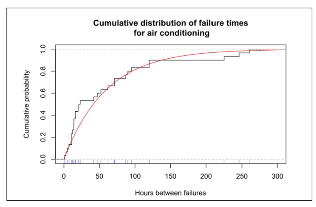
Figure 1 Cumulative distribution function of uptime for air conditioners

Probability models can be applied to an individual part or component or subsystem, to a collection of related parts (e.g., “the hydraulic system”), or to an entire machine. Any of these can be described by the probability distribution of the time before they fail.

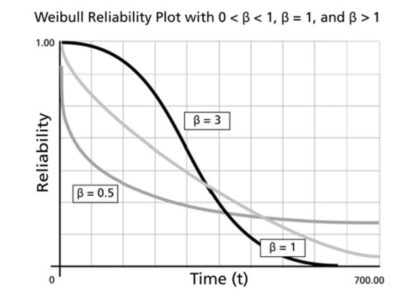
Figure 2 shows the reliability function of six subsystems in a machine for digging tunnels. The plot shows that the most reliable subsystem is the cutting arms and the least reliable is the water subsystem. The reliability of the entire system could be approximated by multiplying all six curves (because for the system as a whole to work, every subsystem must be functioning), which would result in a very short interval before something goes wrong.

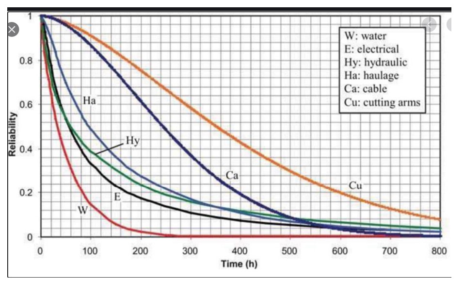
Figure 2 Examples of probability distributions of subsystems in a tunneling machine

Various factors influence the distribution of the time before failure. Investing in better parts will prolong system life. So will investing in redundancy. So will replacing used pars with new.

Once a probability distribution is available, it can be used to answer any number of what-if questions, as illustrated below in the section on Benefits of Models.

Approaches to Modeling Machine Reliability

Probability models can describe either the most basic units, such as individual system components (Figure 2), or collections of basic units, such as entire machines (Figure 1). In fact, an entire machine can be modeled either as a single unit or as a collection of components. If treating an entire machine as a single unit, the probability distribution of lifetime represents a summary of the combined effect of the lifetime distributions of each component.

If we have a model of an entire machine, we can jump to models of collections of machines. If instead we start with models of the lifetimes of individual components, then we must somehow combine those individual models into an overall model of the entire machine.

This is where the math can get hairy. Modeling always requires a wise balance between simplification, so that some results are possible, and complication, so that whatever results emerge are realistic. The usual trick is to assume that failures of the individual pieces of the system occur independently.

If we can assume failures occur independently, it is usually possible to model collections of machines. For instance, suppose a production line has four machines churning out the same product. Having a reliability model for a single machine (as in Figure 1) lets us predict, for instance, the chance that only three of the machines will still be working one week from now. Even here there can be a complication: the chance that a machine working today will still be working tomorrow often depends on how long it has been since its last failure. If the time between failures has an exponential distribution like the one in Figure 1, then it turns out that the time of the next failure doesn’t depend on how long it has been since the last failure. Unfortunately, many or even most systems do not have exponential distributions of uptime, so the complication remains.

Even worse, if we start with models of many individual component reliabilities, working our way up to predicting failure times for the entire complex machine may be nearly impossible if we try to work with all the relevant equations directly. In such cases, the only practical way to get results is to use another style of modeling: Monte Carlo simulation.

Monte Carlo simulation is a way to substitute computation for analysis when it is possible to create random scenarios of system operation. Using simulation to extrapolate machine reliability from component reliabilities works as follows.

1. Start with the cumulative distribution functions (Figure 1) or reliability functions (Figure 2) of each machine component.
2. Create a random sample from each component lifetime to get a set of sample failure times consistent with its reliability function.
3. Using the logic of how components are related to one another, compute the failure time of the entire machine.
4. Repeat steps 1-3 many times to see the full range of possible machine lifetimes.
5. Optionally, average the results of step 4 to summarize the machine lifetime with such metrics such as the MTBF or the chance that the machine will run more than 500 hours before failing.

Step 1 would be a bit complicated if we do not have a nice probability model for a component lifetime, e.g., something like the red line in Figure 1.

Step 2 can require some careful bookkeeping. As time moves forward in the simulation, some components will fail and be replaced while others will keep grinding on. Unless a component’s lifetime has an exponential distribution, its remaining lifetime will depend on how long the component has been in continual use. So this step must account for the phenomena of burn in or wear out.

Step 3 is different from the others in that it does require some background math, though of a simple type. If Machine A only works when both components 1 and 2 are working, then (assuming failure of one component does not influence failure of the other)

Probability [A works] = Probability [1 works] x Probability [2 works].

If instead Machine A works if either component 1 works or component 2 works or both work, then

Probability [A fails] = Probability [1 fails] x Probability [2 fails]

so Probability [A works] = 1 – Probability [A fails].

Step 4 can involve creation of thousands of scenarios to show the full range of random outcomes. Computation is fast and cheap.

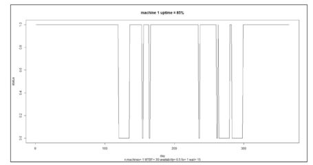
Step 5 can vary depending on the user’s goals. Computing the MTBF is standard. Choose others to suit the problem. Besides the summary statistics provided by step 5, individual simulation runs can be plotted to build intuition about the random dynamics of machine uptime and downtime. Figure 3 shows an example for a single machine showing alternating cycles of uptime and downtime resulting in 85% uptime.

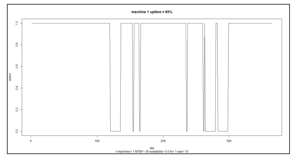
Figure 3 A sample scenario for a single machine

Benefits of Machine Reliability Models

In Figure 3, the machine is up and running 85% of the time. That may not be good enough. You may have some ideas about how to improve the machine’s reliability, e.g., maybe you can improve the reliability of component 3 by buying a newer, better version from a different supplier. How much would that help? That is hard to guess: component 3 may only one of several and perhaps not the weakest link, and how much the change pays off depends on how much better the new one would be. Maybe you should develop a specification for component 3 that you can then shop to potential suppliers, but how long does component 3 have to last to have a material impact on the machine’s MTBF?

This is where having a model pays off. Without a model, you’re relying on guesswork. With a model, you can turn speculation about what-if situations into accurate estimates. For instance, you could analyze how a 10% increase in MTBF for component 3 would translate into an improvement in MTBF for the entire machine.

As another example, suppose you have seven machines producing an important product. You calculate that you must dedicate six of the seven to fill a major order from your one big customer, leaving one machine to handle demand from a number of miscellaneous small customers and to serve as a spare. A reliability model for each machine could be used to estimate the probabilities of various contingencies: all seven machines work and life is good; six machines work so you can at least keep your key customer happy; only five machines work so you have to negotiate something with your key customer, etc.

In sum, probability models of machine or component failure can provide the basis for converting failure time data into smart business decisions.

Read more about  Maximize Machine Uptime with Probabilistic Modeling

Read more about   Probabilistic forecasting for intermittent demand