You may remember the story of Goldilocks from your long-ago youth. Sometimes the porridge was too hot, sometimes it was too cold, but just once it was just right. Now that we are adults, we can translate that fairy tale into a professional principle for inventory planning: There can be too little or too much inventory, and there is some Goldilocks level that is “just right.” This blog is about finding that sweet spot.

To illustrate our supply chain fable, consider this example. Imagine that you sell service parts to keep your customers systems up and running. You offer a particular service part that costs you $100 to make but sells for a 20% markup. You can make $20 on each unit you sell, but you don’t get to keep the whole $20 because of the inventory operating costs you bear to be able to sell the part. There are holding costs to keep the part in good repair while in stock and ordering costs to replenish units you sell. Finally, sometimes you lose revenue from lost sales due to stockouts.  

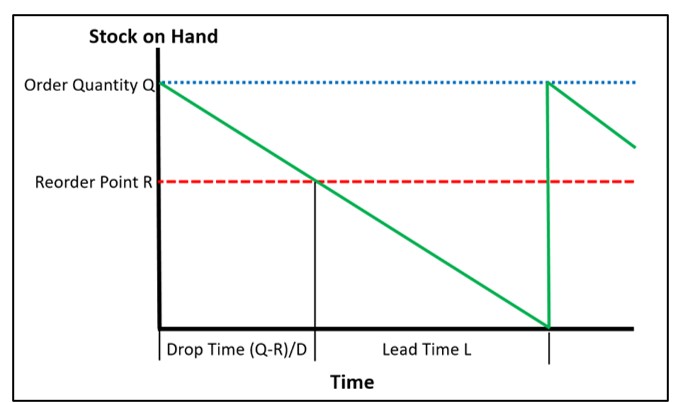
These operating costs can be directly related to the way you manage the part in inventory. For our example, assume you use a (Q,R) inventory policy, where Q is the replenishment order quantity and R is the reorder point. Assume further that the reason you are not making $30 per unit is that you have competitors, and customers will get the part from them if they can’t get it from you.

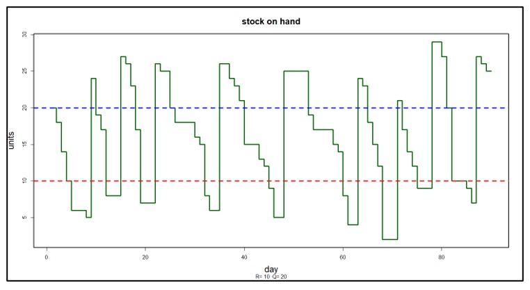
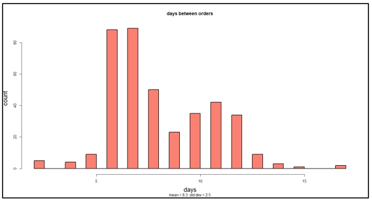
Both your revenue and your costs depend in complex ways on your choices for Q and R. These will determine how much you order, when and therefore how often you order, how often you stock out and therefore how many sales you lose, and how much cash you tie up in inventory. It is impossible to cost out these relationships by guesswork, but modern software can make the relationships visible and calculate the dollar figures you need to guide your choice of values for Q and R. It does this by running detailed, fact-based, probabilistic simulations that predict costs and performance by averaging over a large number of realistic demand scenarios.  

With these results in hand, you can work out the margin associated with (Q,R) values using the simple formula

Margin = (Demand – Lost Sales) x Profit per unit sold – Ordering Costs – Holding Costs.

In this formula, Lost Sales, Ordering Costs and Holding Costs are dependent on reorder point R and order quantity Q.

Figure 1 shows the result of simulations that fixed Q at 25 units and varied R from 10 to 30 in steps of 5. While the curve is rather flat on top, you would make the most money by keeping on-hand inventory around 25 units (which corresponds to setting R = 20). More inventory, despite a higher service level and fewer lost sales, would make a little less money (and ties up a lot more cash), and less inventory would make a lot less.

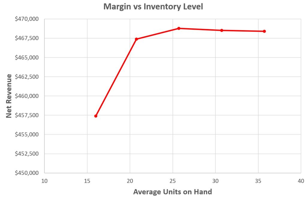
Figure 1: Showing that there can be too little or too much inventory on hand

Without relying on the inventory simulation software, we would not be able to discover

• a) that it is possible to carry too little and too much inventory
• b) what the best level of inventory is
• c) how to get there by proper choices of reorder point R and order quantity Q.

Without an explicit understanding of the above, companies will make daily inventory decisions relying on gut feel and averaging based rule of thumb methods. The tradeoffs described here are not exposed and the resulting mix of inventory yields a far lower return forfeiting hundreds of thousands to millions per year in lost profits.  So be like Goldilocks.  With the right systems and software tools, you too can get it just right!    

Managing the inventory in a single facility is difficult enough, but the problem becomes much more complex when there are multiple facilities arrayed in multiple echelons. The complexity arises from the interactions among the echelons, with demands at the lower levels bubbling up and any shortages at the higher levels cascading down.

If each of the facilities were to be managed in isolation, standard methods could be used, without regard to interactions, to set inventory control parameters such as reorder points and order quantities. However, ignoring the interactions between levels can lead to catastrophic failures. Experience and trial and error allow the design of stable systems, but that stability can be shattered by changes in demand patterns or lead times or by the addition of new facilities. Coping with such changes is greatly aided by advanced supply chain analytics, which provide a safe “sandbox” within which to test out proposed system changes before deploying them. This blog illustrates that point.

The Scenario

To have some hope of discussing this problem usefully, this blog will simplify the problem by considering the two-level hierarchy pictured in Figure 1. Imagine the facilities at the lower level to be warehouses (WHs) from which customer demands are meant to be satisfied, and that the inventory items at each WH are service parts sold to a wide range of external customers.

Figure 1: General structure of one type of two-level inventory system

Imagine the higher level to consist of a single distribution center (DC) which does not service customers directly but does replenish the WHs. For simplicity, assume the DC itself is replenished from a Source that always has (or makes) sufficient stock to immediately ship parts to the DC, though with some delay. (Alternatively, we could consider the system to have retail stores supplied by one warehouse).

Each level can be described in terms of demand levels (treated as random), lead times (random), inventory control parameters (here, Min and Max values) and shortage policy (here, backorders allowed).

The Method of Analysis

The academic literature has made progress on this problem, though usually at the cost of simplifications necessary to facilitate a purely mathematical solution. Our approach here is more accessible and flexible: Monte Carlo simulation. That is, we build a computer program that incorporates the logic of the system operation. The program “creates” random demand at the WH level, processes the demand according to the logic of a chosen inventory policy, and creates demand for the DC by pooling the random requests for replenishment made by the WHs. This approach lets us observe many simulated days of system operation while watching for significant events like stockouts at either level.

An Example

To illustrate an analysis, we simulated a system consisting of four WHs and one DC. Average demand varied across the WHs. Replenishment from the DC to any WH took from 4 to 7 days, averaging 5.15 days. Replenishment of the DC from the Source took either 7, 14, 21 or 28 days, but 90% of the time it was either 21 or 28 days, making the average 21 days. Each facility had Min and Max values set by analyst judgement after some rough calculations.

Figure 2 shows the results of one year of simulated daily operation of this system. The first row in the figure shows the daily demand for the item at each WH, which was assumed to be “purely random”, meaning it had a Poisson distribution. The second row shows the on-hand inventory at the end of each day, with Min and Max values indicated by blue lines. The third row describes operations at the DC.  Contrary to the assumption of much theory, the demand into the DC was not close to being Poisson, nor was the demand out of the DC to the Source. In this scenario, Min and Max values were sufficient to keep item availability was high at each WH and at the DC, with no stockouts observed at any of the five facilities.

Click here to enlarge the image

Figure 2 – Simulated year of operation of a system with four WHs and one DC.

Now let’s vary the scenario. When stockouts are extremely rare, as in Figure 2, there is often excess inventory in the system. Suppose somebody suggests that the inventory level at the DC looks a bit fat and thinks it would be good idea to save money there. Their suggestion for reducing the stock at the DC is to reduce the value of the Min at the DC from 100 to 50. What happens? You could guess, or you could simulate.

Figure 3 shows the simulation – the result is not pretty. The system runs fine for much of the year, then the DC runs out of stock and cannot catch up despite sending successively larger replenishment orders to the Source. Three of the four WHs descend into death spirals by the end of the year (and WH1 follows thereafter). The simulation has highlighted a sensitivity that cannot be ignored and has flagged a bad decision.

Click here to enlarge image

Figure 3 – Simulated effects of reducing the Min at the DC.

Now the inventory managers can go back to the drawing board and test out other possible ways to reduce the investment in inventory at the DC level. One move that always helps, if you and your supplier can jointly make it happen, is to create a more agile system by reducing replenishment lead time. Working with the Source to insure that the DC always gets its replenishments in either 7 or 14 days stabilizes the system, as shown in Figure 4.

Click here to enlarge image

Figure 4 – Simulated effects of reducing the lead time for replenishing the DC.

Unfortunately, the intent of reducing the inventory at the DC has not been achieved. The original daily inventory count was about 80 units and remains about 80 units after reducing the DC’s Min and drastically improving the Source-to-DC lead time. But with the simulation model, the planning team can try out other ideas until they arrive at a satisfactory redesign. Or, given that Figure 4 shows the DC inventory starting to flirt with zero, they might think it prudent to accept the need for an average of about 80 units at the DC and look for ways to trim inventory investment at the WHs instead.

The Takeaways

1. Multiechelon inventory optimization (MEIO) is complex. Many factors interact to produce system behaviors that can be surprising in even simple two-level systems.
2. Monte Carlo simulation is a useful tool for planners who need to design new systems or tweak existing systems.

For most small-to-medium manufacturers and distributors, single-level or single-echelon inventory optimization is at the cutting edge of logistics practice. Multi-echelon inventory optimization (“MEIO”) involves playing the game at an even higher level and is therefore much less common. This blog is the first of two. It aims to explain what MEIO is, why standard MEIO theories break down, and how probabilistic modeling through scenario simulation can restore reality to the MEIO process. The second blog will show a particular example.

Definition of Inventory Optimization

An inventory system is built on a set of design choices.

The first choice is the policy for responding to stockouts: Do you just lose the sale to a competitor, or can you convince the customer to accept a backorder? The former is more common with distributors than manufacturers, but this may not be much of a choice since customers may dictate the answer.

The second choice is the inventory policy. These divide into “continuous review” and “periodic review” policies, with several options within each type. You can link to a video tutorial describing several common inventory policies here.  Perhaps the most efficient is known to practitioners as “Min/Max” and to academics as (s, S) or “little S, Big S.” We use this policy in the scenario simulations below. It works as follows: When on-hand inventory drops to or below the Min (s), an order is placed for replenishment. The size of the order is the gap between the on-hand inventory and the Max (S), so if Min is 10, Max is 25 and on-hand is 8, it’s time for an order of 25-8 = 17 units.

The third choice is to decide on the best values of the inventory policy “parameters”, e.g., the values to use for Min and Max. Before assigning numbers to Min and Max, you need clarity on what “best” means for you. Commonly, best means choices that minimize inventory operating costs subject to a floor on item availability, expressed either as Service Level or Fill Rate. In mathematical terms, this is a “two-dimensional constrained integer optimization problem”. “Two-dimensional” because you have to pick two numbers: Min and Max. “Integer” because Min and Max have to be whole numbers. “Constrained” because you must pick Min and Max values that give a high-enough level of item availability such as service levels and fill rates. “Optimization” because you  want to get there with the lowest operating cost (operating cost combines holding, ordering and shortage costs).

Multiechelon Inventory Systems

The optimization problem becomes more difficult in multi-echelon systems. In a single-echelon system, each inventory item can be analyzed in isolation: one pair of Min/Max values per SKU. Because there are more parts to a multiechelon system, there is a bigger computational problem.

Figure 1 shows a simple two-level system for managing a single SKU. At the lower level, demands arrive at multiple warehouses. When those are in danger of stocking out, they are resupplied from a distribution center (DC). When the DC itself is in danger of stocking out, it is supplied by some outside source, such as the manufacturer of the item.

The design problem here is multidimensional: We need Min and Max values for 4 warehouses and for the DC, so the optimization occurs in 4×2+1×2=10 dimensions. The analysis must take account of a multitude of contextual factors:

• The average level and volatility of demand coming into each warehouse.
• The average and variability of replenishment lead times from the DC.
• The average and variability of replenishment lead times from the source.
• The required minimum service level at the warehouses.
• The required minimum service level at the DC.
• The holding, ordering and shortage costs at each warehouse.
• The holding, ordering and shortage costs at the DC.

As you might expect, seat-of-the-pants guesses won’t do well in this situation. Neither will trying to simplify the problem by analyzing each echelon separately. For instance, stockouts at the DC increase the risk of stockouts at the warehouse level and vice versa.

This problem is obviously too complicated to try to solve without help from some sort of computer model.

Why Standard Inventory Theory is Bad Math

With a little looking, you can find models, journal articles and book about MEIO. These are valuable sources of information and insight, even numbers. But most of them rely on the expedient of over-simplifying the problem to make it possible to write and solve equations. This is the “Fantasy” referred to in the title.

Doing so is a classic modeling maneuver and is not necessarily a bad idea. When I was a graduate student at MIT, I was taught the value of having two models: a small, rough model to serve as a kind of sighting scope and a larger, more accurate model to produce reliable numbers. The smaller model is equation-based and theory-based; the bigger model is procedure-based and data-based, i.e., a detailed system simulation. Models based on simple theories and equations can produce bad numerical estimates and even miss whole phenomena. In contrast, models based on procedures (e.g., “order up to the Max when you breach the Min”) and facts (e.g., the last 3 years of daily item demand) will require a lot more computing but give more realistic answers. Luckily, thanks to the cloud, we have a lot of computing power at our fingertips.

Perhaps the greatest modeling “sin” in the MEIO literature is the assumption that demands at all echelons can be modeled as purely random Poisson processes. Even if it were true at the warehouse level, it would be far from true at the DC level. The Poisson process is the “white rat of demand modeling” because it is simple and permits more paper-and-pencil equation manipulation. Since not all demands are Poisson shaped, this results in unrealistic recommendations.

Scenario-based Simulation Optimization

To get realism, we must get down into the details of how the inventory systems operate at each echelon. With few limits except those imposed by hardware such as size of memory, computer programs can keep up any level of complexity. For instance, there is no need to assume that each of the warehouses faces identical demand streams or has the same costs as all the others.

A computer simulation works as follows.

1. The real-world demand history and lead time history are gathered for each SKU at each location.
2. Values of inventory parameters (e.g., Min and Max) are selected for trial.
3. The demand and replenishment histories are used to create scenarios depicting inputs to the computer program that encodes the rules of operation of the system.
4. The inputs are used to drive the operation of a computer model of the system with the chosen parameter values over a long period, say one year.
5. Key performance indicators (KPI’s) are calculated for the simulated year.
6. Steps 2-5 are repeated many times and the results averaged to link parameter choices to system performance.
7.  

Inventory optimization adds another “outer loop” to the calculations by systematically searching over the possible values of Min and Max. Among those parameter pairs that satisfy the item availability constraint, further search identifies the Min and Max values that result in the lowest operating cost.

Figure 1: General structure of one type of two-level inventory system

Stay Tuned for our next Blog

COMING SOON. To see an example of a simulation of the system in Figure 1, read the second blog on this topic

Consider the problem of replenishing inventory. To be specific, suppose the inventory item in question is a spare part. Both you and your supplier will want some sense of how much you will be ordering and when. And your ERP system may be insisting that you let it in on the secret too.

Deterministic Model of Replenishment

The simplest way to get a decent answer to this question is to assume the world is, well, simple. In this case, simple means “not random” or, in geek speak, “deterministic.” In particular, you pretend that the random size and timing of demand is really a continuous drip-drip-drip of a fixed size coming at a fixed interval, e.g., 2, 2, 2, 2, 2, 2… If this seems unrealistic, it is. Real demand might look more like this: 0, 1, 10, 0, 1, 0, 0, 0 with lots of zeros, occasional but random spikes.

But simplicity has its virtues. If you pretend that the average demand occurs every day like clockwork, it is easy to work out when you will need to place your next order, and how many units you will need.  For instance, suppose your inventory policy is of the (Q,R) type, where Q is a fixed order quantity and R is a fixed reorder point. When stock drops to or below the reorder point R, you order Q units more. To round out the fantasy, assume that the replenishment lead time is also fixed: after L days, those Q new units will be on the shelf ready to satisfy demand.

All you need now to answer your questions is the average demand per day D for the item. The logic goes like this:

1. You start each replenishment cycle with Q units on hand.
2. You deplete that stock by D units per day.
3. So, you hit the reorder point R after (Q-R)/D days.
4. So, you order every (Q-R)/D days.
5. Each replenishment cycle lasts (Q-R)/D + L days, so you make a total of 365D/(Q-R+LD) orders per year.
6. As long as lead time L < R/D, you will never stock out and your inventory will be as small as possible.

Figure 1 shows the plot of on-hand inventory vs time for the deterministic model. Around Smart Software, we refer to this plot as the “Deterministic Sawtooth.” The stock starts at the level of the last order quantity Q. After steadily decreasing over the drop time (Q-R)/D, the level hits the reorder point R and triggers an order for another Q units. Over the lead time L, the stock drops to exactly zero, then the reorder magically arrives and the next cycle begins.

Figure 1: Deterministic model of on-hand inventory

This model has two things going for it. It requires no more than high school algebra, and it combines (almost) all the relevant factors to answer the two related questions: When will we have to place the next order? How many orders will we place in a year?

Probabilistic Model of Replenishment

Not surprisingly, if we strip away some of the fantasy from the deterministic model, we get more useful information. The probabilistic model incorporates all the messy randomness in the real-world problem: the uncertainty in both the timing and size of demand, the variation in replenishment lead time, and the consequences of those two factors: the chance of stock on hand undershooting the reorder point, the chance that there will be a stockout, the variability in the time until the next order, and the variable number of orders executed in a year.

The probabilistic model works by simulating the consequences of uncertain demand and variable lead time. By analyzing the item’s historical demand patterns (and excluding any observations that were recorded during a time when demand may have been fundamentally different), advanced statistical methods create an unlimited number of realistic demand scenarios. Similar analysis is applied to records of supplier lead times. Combining these supply and demand scenarios with the operational rules of any given inventory control policy produces scenarios of the number of parts on hand. From these scenarios, we can extract summaries of the varying intervals between orders.

Figure 2 shows an example of a probabilistic scenario; demand is random, and the item is managed using reorder point R = 10 and order quantity Q=20. Gone is the Deterministic Sawtooth; in its place is something more complex and realistic (the Probabilistic Staircase). During the 90 simulated days of operation, there were 9 orders placed, and the time between orders clearly varied.

Using the probabilistic model, the answers to the two questions (how long between orders and how many in a year) get expressed as probability distributions reflecting the relative likelihoods of various scenarios. Figure 3 shows the distribution of the number of days between orders after ten years of simulated operation. While the average is about 8 days, the actual number varies widely, from 2 to 17.

Instead of telling your supplier that you will place X orders next year, you can now project X ± Y orders, and your supplier knows better their upside and downside risks. Better yet, you could provide the entire distribution as the richest possible answer.

Figure 2 A probabilistic scenario of on-hand inventory

Figure 3: Distribution of days between orders

Climbing the Random Staircase to Greater Efficiency

Moving beyond the deterministic model of  inventory opens up new possibilities for optimizing operations. First, the probabilistic model allows realistic assessment of stockout risk. The simple model in Figure 1 implies there is never a stockout, whereas probabilistic scenarios allow for the possibility (though in Figure 2 there was only one close call around day 70). Once the risk is known, software can optimize by searching  the “design space” (i.e., all possible values of R and Q) to find a design that meets a target level of stockout risk at minimal cost. The value of the deterministic model in this more realistic analysis is that it provides a good starting point for the search through design space.

Summary

Modern software provides answers to operational questions with various degrees of detail. Using the example of the time between replenishment orders, we’ve shown that the answer can be calculated approximately but quickly by a simple deterministic model. But it can also be provided in much richer detail with all the variability exposed by a probabilistic model. We think of these alternatives as complementary. The deterministic model bundles all the key variables into an easy-to-understand form. The probabilistic model provides additional realism that professionals expect and supports effective search for optimal choices of reorder point and order quantity.