Our customers have usually settled into one way to manage their service parts inventory. The professor in me would like to think that the chosen inventory policy was a reasoned choice among considered alternatives, but more likely it just sort of happened. Maybe the inventory honcho from long ago had a favorite and that choice stuck. Maybe somebody used an EAM or ERP system that offered only one choice. Perhaps there were some guesses made, based on the conditions at the time.

The Competitors

Too seldom, businesses make these choices in haphazard ways. But modern service parts planning software lets you be more systematic about your choices. This post demonstrates that proposition by making objective comparisons among three popular inventory policies:  Order Up To, Reorder Point/Order Quantity, and Min/Max.  I discussed each of these policies in this video blog.

• Order Up To. This is a periodic review policy where every T days, on-hand inventory is tallied and an order of random size is placed to bring the stock level back up to S units.
• Q, R or Reorder Point/Order Quantity. Q, R is a continuous review policy where every day, inventory is tallied. If there are Q or fewer units on hand, an order of fixed size is placed for R more units.
• Min, Max is another continuous review policy where every day, inventory is tallied. If there are Min or fewer units on hand, an order is placed to bring the stock level back up to Max units.

Inventory theory says these choices are listed in increasing order of effectiveness. The first option, Order Up To, is clearly the simplest and cheapest to implement, but it closes its eyes to what’s going on for long periods of time.  Imposing a specified passage of time in between orders makes it, in theory, less flexible. In contrast, the two continuous review options keep an eye on what’s happening all the time, so they can react to potential stockouts quicker. The Min/Max option is, in theory, more flexible than the option that uses a fixed reorder quantity because the size of the order dynamically changes to accommodate the demand.

That’s the theory. This post examines evidence from head-to-head comparisons to check the theory and put concrete numbers on the relative performance of the three policies.

The Meaning of “Best”

How should we keep score in this tournament? If you are a regular reader of this Smart Forecaster blog, you know that the core of inventory planning is a tug-of-war between two opposing objectives: keeping inventory lean vs keeping item availability metrics such as service level high.

To simplify things, we will compute “one number to rule them all”: the average operating cost. The winning policy will be the one with the lowest average.

This average is the sum of three components: the cost of holding inventory (“holding cost”), the cost of ordering replenishment units (“ordering cost”) and the cost of losing a sale (“shortage cost”). To make things concrete, we used the following assumptions:

• Each service part is valued at $1,000.
• Annual holding cost is 10% of item value, or $100 per year per unit.
• Processing each replenishment order costs $20 per order.
• Each unit demanded but not provided costs the value of the part, $1,000.

For simplicity, we will refer to the average operating cost as simply “the cost”.

Of course, the lowest average cost can be achieved by getting out of the business. So the competition required a performance constraint on item availability: Each option had to achieve a fill rate of at least 99%.

The Alternatives Duke it Out

A key element of context is whether stockouts result in losses or backorders. Assuming that the service part in question is critical, we assumed that unfilled orders are lost, which means that a competitor fills the order. In an MRO environment, this will mean additional downtime due to stockout.

To compare the alternatives, we used our predictive modeling engine to run a large number of Monte Carlo simulations.  Each simulation involved specifying the parameter values of each policy (e.g., Min and Max values), generating a demand scenario, feeding that into the logic of the policy, and measuring the resulting cost averaged over 365 days of operation. Repeating this process 1,000 times and averaging the 1,000 resulting costs gave the final result for each policy.  

To make the comparison fair, each alternative had to be designed for its best performance. So we searched the “design space” of each policy to find the design with the lowest cost. This required repeating the process described in the previous paragraph for many pairs of parameter values and identifying the pair yielding the lost average annual operating cost.

Using the algorithms in Smart Inventory Optimization (SIO^TM) we made head-to-head-to-head comparisons under the following assumptions about demand and supply:

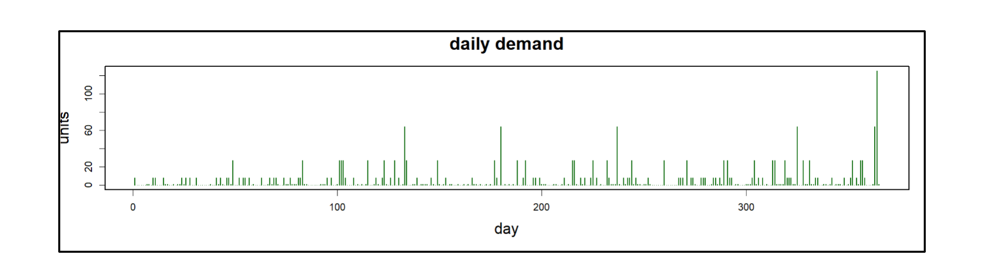
• Item demand was assumed to be intermittent and highly variable but relatively simple in that there was neither trend nor seasonality, as is often true for service parts. Daily mean demand was 5 units with a large standard deviation of 13 units. Figure 1 shows a sample of one year’s demand. We have chosen a very challenging demand pattern, in which some days have 10 to even 20 times the average demand.

Figure 1: Daily part demand was assumed to be intermittent and very spikey.

​​

• Suppliers’ replenishment lead times were 14 days 75% of the time and 21 days otherwise. This reflects the fact that there is always uncertainty in the supply chain.

And the Winner Is…

Was the theory right? Kinda’ sorta’.

Table 1 shows the results of the simulation experiments. For each of the three competing policies, it shows the average annual operating cost, the margin of error (technically, an approximate 95% confidence interval for the mean cost), and the apparent best choices for parameter values.

Table 1: Results of the simulated comparisons

For example, the average cost for the (T,S) policy when T is fixed at 30 days was $41,680. But the Plus/Minus implies that the results are compatible with a “true” cost (i.e., the estimate from an infinite number of simulations) of anywhere between $39,890 and $43,650. The reason there is so much statistical uncertainty is the extremely spikey nature of demand in this example.

Table 1 says that, in this example, the three policies fall in line with expectations. However, more useful conclusions would be:

1. The three policies are remarkably similar in average cost. By clever choice of parameter values, one can get good results out of any of the three policies.
2. Not shown in Table 1, but clear from the detailed simulation results, is that poor choices for parameter values can be disastrous for any policy.
3. It is worth noting that the periodic review (T,S) policy was not allowed to optimize over possible values of T. We fixed T at 30 to mimic what is common in practice, but those who use the periodic review policy should consider other review periods. An additional experiment fixed the review period at T = 7 days. The average cost in this scenario was minimized at $36,551 ± $1,668 with S = 343. This result is better than that using T = 30 days.
4. We should be careful about over-generalizing these results. They depend on the assumed values of the three cost parameters (holding, ordering and shortage) and the character of the demand process.
5. It is possible to run experiments like those shown here automatically in Smart Inventory Optimization. This means that you too would be able to explore design choices in a rigorous way.

In almost every business and industry, decision-makers need reliable forecasts of critical variables, such as sales, revenues, product demand, inventory levels, market share, expenses, and industry trends.

Many kinds of people make these forecasts. Some are sophisticated technical analysts, such as business economists and statisticians. Many others regard forecasting as an important part of their overall work: general managers, production planners, inventory control specialists, financial analysts, strategic planners, market researchers, and product and sales managers. Still, others seldom think of themselves as forecasters but often have to make forecasts on an intuitive, judgmental basis.

Because of the way we designed Smart Demand Planner, it has something to offer all types of forecasters. This design grows out of several observations about the forecasting process. Because we designed Smart Demand Planner with these observations in mind, we believe it has a style and content uniquely suited for turning your browser into an effective forecasting and planning tool:

Forecasting is an art that requires a mix of professional judgment and objective, statistical analysis.

It is often effective to begin with an objective statistical forecast that automatically accounts for trends, seasonality, and other patterns.  Then, apply adjustments or forecast overrides based on your business judgment. Smart Demand Planner makes it easy to execute graphical and tabular adjustments to statistical forecasts.

The forecasting process is usually iterative.

You will likely decide to make several refinements of your initial forecast before you are satisfied. You may want to exclude older historical data that you find to no longer be relevant.  You could apply different weights to the forecast model that put varying emphases on the most recent data. You could apply trend dampening to increase or decrease aggressively trending statistical forecasts.  You could allow the Machine Learning models to fine-tune the forecast selection for you and select the winning model automatically.  Smart Demand Planner’s processing speed gives you plenty of time to make several passes and saves multiple versions of the forecasts as “snapshots” so you can compare forecast accuracy later.

Forecasting requires graphical support.

The patterns evident in data can be seen by a discerning eye. The credibility of your forecasts will often depend heavily on graphical comparisons other business stakeholders make when they assess the historical data and forecasts. Smart Demand Planner provides graphical displays of forecasts, history, and forecast vs. actuals reporting.

Forecasts are never exactly correct.

Because some error always creeps into even the best forecasting process, one of the most useful supplements to a forecast is an honest estimate of its margin of error.

Smart Demand Planner presents both graphical and tabular summaries of forecast accuracy based on the acid test of predicting data held back from development of the forecasting model. 

Forecast intervals or confidence intervals are also very useful.  They detail the likely range of possible demand that is expected to occur.  For example, if actual demand falls outside of the 90% confidence interval more than 10% of the time then there is reason to investigate further.  

Forecasting requires a match of method to data.

One of the major technical tasks in forecasting is to match the choice of forecasting technique to the nature of the data. Features of a data series like trend, seasonality or abrupt shifts in level suggest certain techniques instead of others.

Smart Demand Planner’ Automatic forecasting feature makes this match quickly, accurately and automatically.

Forecasting is often a part of a larger process of planning or control.

For example, forecasting can be a powerful complement to spreadsheet-based financial analysis, extending rows of figures off into the future. In addition, accurate sales and product demand forecasts are fundamental inputs to a manufacturer’s production planning and inventory control processes. An objective statistical forecast of future sales will always help identify when the budget (or sales plan) may be too unrealistic. Gap analysis enables the business to take corrective action to their demand and marketing plans to ensure they do not miss the budgeted plan.

Forecasts need to be integrated into ERP systems
Smart Demand Planner can quickly and easily transfer its results to other applications, such as spreadsheets, databases and planning systems including ERP applications.  Users are able to export forecasts in a variety of file formats either via download or to secure FTP file locations.  Smart Demand Planner includes API based integrations to a variety of ERP and EAM systems including Epicor Kinetic and Epicor Prophet 21, Sage X3 and Sage 300, Oracle NetSuite, and each of Microsoft’s Dynamics 365 ERP systems. API based integrations enable customers to push forecast results directly back to the ERP system on demand.

The result is more efficient sales planning, budgeting, production scheduling, ordering, and inventory planning.

In this article, we will review the “suggested orders” functionality in Epicor BisTrack, explain its limitations, and summarize how Smart Inventory Planning & Optimization (Smart IP&O) can help reduce inventory & minimize stock-outs by accurately assessing the tradeoffs between stockout risks and inventory costs.

Automating Replenishment in Epicor BisTrack
Epicor BisTrack’s “Suggested Ordering” can manage replenishment by suggesting what to order and when via reorder point-based policies such as min-max and/or manually specified weeks of supply. BisTrack contains some basic functionality to compute these parameters based on average usage or sales, supplier lead time, and/or user-defined seasonal adjustments. Alternatively, reorder points can be specified completely manually. BisTrack will then present the user with a list of suggested orders by reconciling incoming supply, current on hand, outgoing demand, and stocking policies.

How Epicor BisTrack “Suggested Ordering” Works
To get a list of suggested orders, users specify the methods behind the suggestions, including locations for which to place orders and how to determine the inventory policies that govern when a suggestion is made and in what quantity.

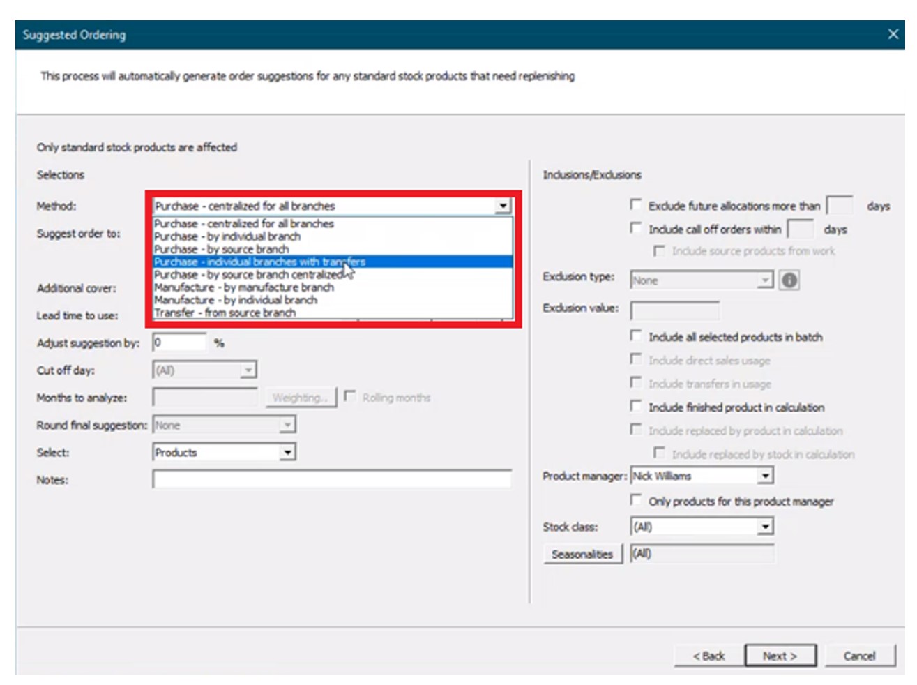
First, the “method” field is specified from the following options to determine what kind of suggestion is generated and for which location(s):

Purchase – Generate purchase order recommendations.

1. Centralized for all branches – Generates suggestions for a single location that buys for all other locations.
2. By individual branch – Generates suggestions for multiple locations (vendors would ship directly to each branch).
3. By source branch – Generates suggestions for a source branch that will transfer material to branches that it services (“hub and spoke”).
4. Individual branches with transfers – Generates suggestions for an individual branch that will transfer material to branches that it services (“hub and spoke”, where the “hub” does not need to be a source branch).

Manufacture – Generate work order suggestions for manufactured goods.

1. By manufacture branch.
2. By individual branch.

Transfer from source branch – Generate transfer suggestions from a given branch to other branches.

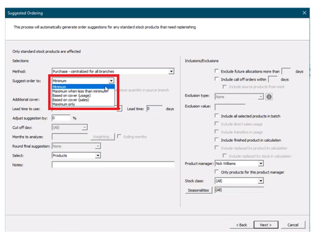
Next, the “suggest order to” is specified from the following options:

1. Minimum – Suggests orders “up to” the minimum on hand quantity (“min”). For any item where supply is less than the min, BisTrack will suggest an order suggestion to replenish up to this quantity.
2. Maximum when less than min – Suggests orders “up to” a maximum on-hand quantity when the minimum on-hand quantity is breached (e.g. a min-max inventory policy).

3. Based on cover (usage) – Suggests orders based on coverage for a user-defined number of weeks of supply with respect to a specified lead time. Given internal usage as demand, BisTrack will recommend orders where supply is less than the desired coverage to cover the difference.

4. Based on over (sales) – Suggests orders based on coverage for a user-defined number of weeks of supply with respect to a specified lead time. Given sales orders as demand, BisTrack will recommend orders where supply is less than the desired coverage to cover the difference.

5. Maximum only – Suggests orders “up to” a maximum on-hand quantity where supply is less than this max.

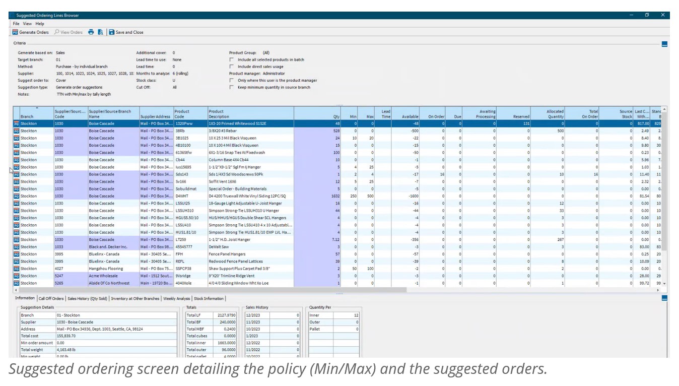
Finally, if allowing BisTrack to determine the reorder thresholds, users can specify additional inventory coverage as buffer stock, lead times, how many months of historical demand to consider, and can also manually define period-by-period weighting schemes to approximate seasonality. The user will be handed a list of suggested orders based on the defined criteria. A buyer can then generate POs for suppliers with the click of a button.

Limitations

Rule-of-thumb Methods

While BisTrack enables organizations to generate reorder points automatically, these methods rely on simple averages that do not capture seasonality, trends, or the volatility in an item’s demand. Averages will always lag behind these patterns and are unable to pick up on trends. Consider a highly seasonal product like a snow shovel—if we take an average of Summer/Fall demand as we approach the Winter season instead of looking ahead, then the recommendations will be based on the slower periods instead of anticipating upcoming demand. Even if we consider an entire years’ worth of history or more, the recommendations will overcompensate during the slower months and underestimate the busy season without manual intervention.

Rule of thumb methods also fail when used to buffer against supply and demand variability.  For example, the average demand over the lead time might be 20 units.  However, a planner would often want to stock more than 20 units to avoid stocking out if lead times are longer than expected or demand is higher than the average.  BisTrack allows users to specify the reorder points based on multiples of the averages.  However, because the multiples don’t account for the level of predictability and variability in the demand, you’ll always overstock predictable items and understock unpredictable ones.   Read this article to learn more about why multiples of the average fail when it comes to developing the right reorder point.

Manual Entry
Speaking of seasonality referenced earlier, BisTrack does allow the user to approximate it through the use of manually entered “weights” for each period. This forces the user to have to decide what that seasonal pattern looks like—for every item. Even beyond that, the user must dictate how many extra weeks of supply to carry to buffer against stockouts, and must specify what lead time to plan around. Is 2 weeks extra supply enough? Is 3 enough? Or is that too much? There is no way to know without guessing, and what makes sense for one item might not be the right approach for all items.

Intermittent Demand
Many BisTrack customers may consider certain items “unforecastable” because of the intermittent or “lumpy” nature of their demand. In other words, items that are characterized by sporadic demand, large spikes in demand, and periods of little or no demand at all. Traditional methods—and rule-of-thumb approaches especially—won’t work for these kinds of items. For example, 2 extra weeks of supply for a highly predictable, stable item might be way too much; for an item with highly volatile demand, this same rule might not be enough. Without a reliable way to objectively assess this volatility for each item, buyers are left guessing when to buy and how much.

Reverting to Spreadsheets
The reality is most BisTrack users tend to do the bulk of their planning off-line, in Excel. Spreadsheets aren’t purpose-built for forecasting and inventory optimization. Users will often bake in user-defined rule of thumb methods that often do more harm than good.  Once calculated, users must input the information back into BisTrack manually. The time consuming nature of the process leads companies to infrequently compute their inventory policies – Many months and on occasion years go by in between mass updates leading to a “set it and forget it” reactive approach, where the only time a buyer/planner reviews inventory policy is at the time of order.  When policies are reviewed after the order point is already breached, it is too late.  When the order point is deemed too high, manual interrogation is required to review history, calculate forecasts, assess buffer positions, and to recalibrate.  The sheer volume of orders means that buyers will just release orders rather than take the painstaking time to review everything, leading to significant excess stock.  If the reorder point is too low, it’s already too late.  An expedite may now be required, driving up costs, assuming the customer doesn’t simply go elsewhere.

Epicor is Smarter
Epicor has partnered with Smart Software and offers Smart IP&O as a cross platform add-on to its ERP solutions including BisTrack, a speciality ERP for the Lumber, hardware, and building material industry.  The Smart IP&O solution comes complete with a bidirectional integration to BisTrack.  This enables Epicor customers to leverage built-for-purpose best of breed inventory optimization applications.  With Epicor Smart IP&O you can generate forecasts that capture trend and seasonality without manual configurations.  You will be able to automatically recalibrate inventory policies using field proven, cutting-edge statistical and probabilistic models that were engineered to accurately plan for intermittent demand.   Safety stocks will accurately account for demand and supply variability, business conditions, and priorities.  You can leverage service level driven planning so you have just enough stock or turn on optimization methods that prescribe the most profitable stocking policies and service levels that consider the real cost of carrying inventory. You can support commodity buys with accurate demand forecasting over longer horizons, and run “what-if” scenarios to assess alternative strategies before execution of the plan.

Smart IP&O customers routinely realize 7 figure annual returns from reduced expedites, increased sales, and less excess stock, all the while gaining a competitive edge by differentiating themselves on improved customer service. To see a recorded webinar hosted by the Epicor Users Group that profiles Smart’s Demand Planning and Inventory Optimization platform, please register here.

​In a highly configurable manufacturing environment, forecasting finished goods can become a complex and daunting task. The number of possible finished products will skyrocket when many components are interchangeable. A traditional MRP would force us to forecast every single finished product which can be unrealistic or even impossible. Several leading ERP solutions introduce the concept of the “Planning BOM”, which allows the use of forecasts at a higher level in the manufacturing process. In this article, we will discuss this functionality in ERP, and how you can take advantage of it with Smart Inventory Planning and Optimization (Smart IP&O) to get ahead of your demand in the face of this complexity.

Why Would I Need a Planning BOM?

Traditionally, each finished product or SKU would have a rigidly defined bill of materials. If we stock that product and want to plan around forecasted demand, we would forecast demand for those products and then feed MRP to blow this forecasted demand from the finished good level down to its components via the BOM.

Many companies, however, offer highly configurable products where customers can select options on the product they are buying. As an example, recall the last time you bought a personal computer. You chose a brand and model, but from there, you were likely presented with options: what speed of CPU do you want? How much RAM do you want? What kind of hard drive and how much space? If that business wants to have these computers ready and available to ship to you in a reasonable time, suddenly they are no longer just anticipating demand for that model—they must forecast that model for every type of CPU, for all quantities of RAM, for all types of hard drive, and all possible combinations of those as well! For some manufacturers, these configurations can compound to hundreds or thousands of possible finished good permutations.

There may be so many possible customizations that the demand at the finished product level is completely unforecastable in a traditional sense. Thousands of those computers may sell every year, but for each possible configuration, the demand may be extremely low and sporadic—perhaps certain combinations sell once and never again.

This often forces these companies to plan reorder points and safety stock levels mostly at the component level, while largely reacting to firm demand at the finished good level via MRP. While this is a valid approach, it lacks a systematic way to leverage forecasts that may account for anticipated future activity such as promotions, upcoming projects, or sales opportunities. Forecasting at the “configured” level is effectively impossible, and trying to weave in these forecast assumptions at the component level isn’t feasible either.

Planning BOM Explained

This is where Planning BOMs come in. Perhaps the sales team is working a big b2b opportunity for that model, or there’s a planned promotion for Cyber Monday. While trying to work in those assumptions for every possible configuration isn’t realistic, doing it at the model level is totally doable—and tremendously valuable.

The Planning BOM can use a forecast at a higher level and then blow demand down based on predefined proportions for its possible components. For example, the computer manufacturer may know that most people opt for 16GB of RAM, and far fewer opt for the upgrades to 32 or 64. The planning BOM allows the organization to (for example) blow 60% of the demand down to the 16GB option, 30% to the 32GB option, and 10% to the 64GB option. They could do the same for CPUs, hard drives, or any other customizations available.  

The business can now focus their forecast at this model level, leaving the Planning BOM to figure out the component mix. Clearly, defining these proportions requires some thought, but Planning BOMs effectively allow businesses to forecast what would otherwise be unforecastable.

The Importance of a Good Forecast

Of course, we still need a good forecast to load into an ERP system. As explained in this article, while ERP  can import a forecast, it often cannot generate one and when it does it tends to require a great deal of hard to use configurations that don’t often get revisited resulting in inaccurate forecasts.  It is therefore up to the business to come up with their own sets of forecasts, often manually produced in Excel. Forecasting manually generally presents a number of challenges, including but not limited to:

• The inability to identify demand patterns like seasonality or trend
• Overreliance on customer or sales forecasts
• Lack of accuracy or performance tracking

No matter how well configured the MRP is with your carefully considered Planning BOMs, a poor forecast means poor MRP output and mistrust in the system—garbage in, garbage out. Continuing along with the “computer company” example, without a systematic way of capturing key demand patterns and/or domain knowledge in the forecast, MRP can never see it.

Extend ERP  with Smart IP&O

Smart IP&O is designed to extend your ERP system with a number of integrated demand planning and inventory optimization solutions. For example, it can generate statistical forecasts automatically for large numbers of items, allows for intuitive forecast adjustments, tracks forecast accuracy, and ultimately allows you to generate true consensus-based forecasts to better anticipate the needs of your customers.

Thanks to highly flexible product hierarchies, Smart IP&O is perfectly suited to forecasting at the Planning BOM level so you can capture key patterns and incorporate business knowledge at the levels that matter most. Furthermore you can analyze and deploy optimal safety stock levels at any level of your BOM.