Two Inventory Problems

If you both make and sell things, you own two inventory problems. Companies that sell things must focus relentlessly on having enough product inventory to meet customer demand.  Manufacturers and asset intensive industries such as power generation, public transportation, mining, and refining, have an additional inventory concern:  having enough spare parts to keep their machines running. This technical brief reviews the basics of two probabilistic models of machine breakdown. It also relates machine uptime to the adequacy of spare parts inventory.

Modeling the failure of a machine treated as a “black box”

Just as product demand is inherently random, so is the timing of machine breakdowns. Likewise, just as probabilistic modeling is the right way to deal with random demand, it is also the right way to deal with random breakdowns.

Models of machine breakdown have two components. The first deals with the random duration of uptime. The second deals with the random duration of downtime.

The field of reliability theory offers several standard probability models describing the random time until failure of a machine without regard for the reason for the failure. The simplest model of uptime is the exponential distribution. This model says that the hazard rate, i.e., the chance of failing in the next instant of time, is constant no matter how long the system has been operating. The exponential model does a good job at modeling certain types of systems, especially electronics, but it is not universally applicable.

Download the Whitepaper

The next step up in model complexity is the Weibull model (pronounced “WHY-bull”). The Weibull distribution allows the risk of failure to change over time, either decreasing after a burn in period or, more often, increasing as wear and tear accumulate. The exponential distribution is a special case of the Weibull distribution in which the hazard rate is neither increasing nor decreasing.

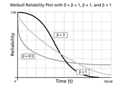
Figure 1: Three different Weibull survival curves

Figure 1 illustrates the Weibull model’s probability that a machine is still running as a function of how long it has been running. There are three curves corresponding to constant, decreasing and increasing hazard rates. For obvious reasons, these are called survival curves because they plot the probability of surviving for various amounts of time (but they are also called reliability curves). The black curve that starts high and sinks fast (β=3) depicts a machine that wears out with age. The lightest curve in the middle fast (β=1) shows the exponential distribution. The medium-dark curve (β=0.5)  is one that has a high early hazard rate but gets better with age.

Of course, there is another phenomenon that needs to be included in the analysis: downtime. Modeling downtime is where inventory theory enters the picture. Downtime is modeled by a mixture of two different distributions. If a spare part is available to replace the failed part, then the downtime can be very brief, say one day. But if there is no spare in stock, then the downtime can be quite long. Even if the spare can be obtained on an expedited basis, it may be several days or a week before the machine can be repaired. If the spare must be fabricated by a far-away supplier and shipped by sea then by rail then trucked to your plant, the downtime could be weeks or months. This all means that keeping a proper inventory of spares is very important to keeping production humming along.

In this aggregated type of analysis, the machine is treated as a black box that is either working or not. Though ignoring the details of which part failed and when, such a model is useful for sizing the pool of machines needed to maintain some minimum level of production capacity with high probability.

The binomial distribution is the probability model relevant to this problem. The binomial is the same model that describes, for example, the distribution of the number of “heads” resulting from twenty tosses of a coin. In the machine reliability problem, the machines correspond to coins, and an outcome of heads corresponds to having a working machine.

As an example, if

• the chance that any given machine is running on any particular day is 90%
• machine failures are independent (e.g., no flood or tornado to wipe them all out at once)
• you require at least a 95% chance that at least 5 machines are running on any given day

then the binomial model prescribes seven machines to achieve your goal.

Modeling machine failures based on component failures

The Weibull model can also be used to describe the failure of a single part. However, any realistically complex production machine will have multiple parts and therefore have multiple failure modes. This means that calculating the time until the machine fails requires analysis of a “race to failure”, with each part vying for the “honor” of being the first to fail.

If we make the reasonable assumption that parts fail independently, standard probability theory points the way to combining the models of individual part failure into an overall model of machine failure. The time until the first of many parts fails has a poly-Weibull distribution. At this point, though, the analysis can get quite complicated, and the best move may be to switch from analysis-by-equation to analysis-by-simulation.

Simulating machine failure from the details of part failures

Simulation analysis got its modern start as a spinoff of the Manhattan Project to build the first atomic bomb. The method is also commonly called Monte Carlo simulation after the biggest gambling center on earth back in the day (today it would be “Macau simulation”).

A simulation model converts the logic of the sequence of random events into corresponding computer code. Then it uses computer-generated (pseudo-)random numbers as fuel to drive the simulation model. For example, each component’s failure time is created by drawing from its particular Weibull failure time distribution. Then the soonest of those failure times begins the next episode of machine downtime.

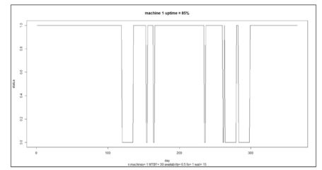
Figure 2: A simulation of machine uptime over one year of operation

Figure 2 shows the results of a simulation of the uptime of a single machine. Machines cycle through alternating periods of uptime and downtime. In this simulation, uptime is assumed to have an exponential distribution with an average duration (MTBF = Mean Time Before Failure) of 30 days. Downtime has a 50:50 split between 1 day if a spare is available and 30 days if not. In the simulation shown in Figure 2, the machine is working during 85% of the days in one year of operation.

An approximate formula for machine uptime

Although Monte Carlo simulation can provide more exact results, a simpler algebraic model does well as an approximation and makes it easier to see how the key variables relate.

Define the following key variables:

• MTBF = Mean Time Before Failure (days)
• Pa = Probability that there is a spare part available when needed
• MDTshort = Mean Down Time if there is a spare available when needed
• MDTlong = Mean Down Time if there is no spare available when needed
• Uptime = Percentage of days in which the machine is up and running.

Then there is a simple approximation for the Uptime:

Uptime ≈ 100 x MTBF/(MTBF + MDTshort x Pa + MDTlong x (1-Pa)).    (Equation 1)

Equation 1 tells us that the uptime depends on the availability of a spare. If there is always a spare (Pa=1), then uptime achieves a peak value of about 100 x MTBF/(MTBF + MDTshort). If there is never a spare available (Pa=0), then uptime achieve its lowest value of about 100 x MTBF/(MTBF + MDTlong). When the repair time is about as long as the typical time between failures, uptime sinks to an unacceptable level near 50%. If a spare is always available, uptime can approach 100%.

Relating machine downtime to spare parts inventory

Minimizing downtime requires a multi-pronged initiative involving intensive operator training, use of quality raw materials, effective preventive maintenance – and adequate spare parts. The first three set the conditions for good results. The last deals with contingencies.

Once a machine is down, money is flying out the door and there is a premium on getting it back up pronto. This scene could play out in two ways. The good one has a spare part ready to go, so the downtime can be kept to a minimum. The bad one has no available spare, so there is a scramble to expedite delivery of the needed part. In this case, the manufacturer must bear both the cost of lost production and the cost of expedited shipping, if that is even an option.

If the inventory system is properly designed, spare parts availability will not be a major impediment to machine uptime. By the design of an inventory system, I mean the results of several choices: whether the shortage policy is a backorder policy or a loss policy, whether the inventory review cycle is periodic or continuous, and what reorder points and order quantities are established.

When inventory policies for products are designed, they are evaluated using several criteria. Service Level is the percentage of replenishment periods that pass without a stockout. Fill Rate is the percentage of units ordered that is supplied immediately from stock. Average Inventory Level is the typical number of units on hand.

None of these is exactly the metric needed for spare parts stocking, though they all are related. The needed metric is Item Availability, which is the percentage of days in which there is at least one spare ready for use. Higher Service Levels, Fill Rates, and Inventory Levels all imply high Item Availability, and there are ways to convert from one to the other. (When dealing with multiple machines sharing the same stock of spares, Inventory Availability gets replaced by the probability distribution of the number of spares on any given day. We leave that more complex problem for another day.)

Clearly, keeping a good supply of spares reduces the costs of machine downtime. Of course, keeping a good supply of spares creates its own inventory holding and ordering costs. This is the manufacturer’s second inventory problem. As with any decision involving inventory, the key is to strike the right balance between these two competing cost centers. See this article on probabilistic forecasting for intermittent demand for guidance on striking that balance.

Service Level Driven Planning (SLDP) is an approach to inventory planning. It prescribes optimal service level targets continually identifies and communicates trade-offs between service and cost that are at the root of all wise inventory decisions. When an organization understands this relationship, they can communicate where they are at risk, where they are not, and effectively wield their inventory assets.  SLDP helps expose inventory imbalances and enables informed decisions on how best to correct them.  To implement SLDP, you’ll need to look beyond traditional planning approaches such as arbitrary service level targeting (all of my A items should get 99% service level, B items 95%, C items 80%, etc.) and demand forecasting that unrealistically attempts to predict exactly what will happen and when. SLDP unfolds in 4 steps: Benchmark, Collaborate, Plan, and Track.

Step 1. Benchmark Performance

All participants in the inventory planning and investment process must hold a common understanding of how current policy is performing across an agreed upon set of inventory metrics. Metrics should include historically achieved service levels and fill rates, delivery time to customers, supplier lead time performance, inventory turns, and inventory investment. Once these metrics have been benchmarked and can be reported on daily, the organization will have the information it needs to begin prioritize planning efforts. For example, if inventory has increased but service levels have not, this would indicate that the inventory is not being properly allocated across SKUs.  Reports should be generated within mouse-clicks enabling planners to focus on analysis instead of time intensive report generation.   Past performance isn’t a guarantee of future performance since demand variability, costs, priorities, and lead times are always changing. So SLDP enables predictive benchmarking that estimates what performance is likely to be in the future. Inventory optimization software utilizing probability forecasting can be used to estimate a realistic range of potential demands and replenishment cycles stress testing your planning parameters helping uncover how often and which items to expect stockouts and excess.

Step 2. “What if” Planning & Collaboration

“What if” inventory modeling and collaboration is at the heart of SLDP. The historical and predictive benchmarks should first be shared with all relevant stakeholders including sales, finance, and operations. Efforts should be placed on answering the following questions:

– Are both the current performance and investment acceptable?
– If not, how should they be improved?
– Which SKUs are likely to be demanded next and in what quantities?
– Where are we willing to take more stock out risk?
– Where must stock-out risk be minimized?
– What are the specific stock out costs?
– What business rules and constraints must we adhere to (customer service level agreements, inventory thresholds, etc.)

Once the above questions are answered, new inventory planning policies can be developed.  Inventory Optimization software can reconcile all costs associated with managing inventory including stockout costs to generate the right set of planning parameters (min/max, safety stock, reorder points, etc.) and prescribed service levels.  The optimal policy can be compared to the current policy and modified based on constraints and business rules. For example, certain items might be targeted at a target service level in order to conform to a customer service level agreement.   Various “what if” inventory planning scenarios can be developed and shared with key stakeholders. For example, you might model how shorter lead times impacts inventory costs. Once consensus has been achieved and the risks and costs are clearly communicated,  the modified policies can be uploaded to the ERP system to drive inventory replenishment.

Step 3. Continually Plan and Manage by Exception

SLDP continually reforecasts optimized planning parameters based on changing demands, lead times, costs, and other factors. This means that service levels and inventory value have the potential to change.  For example, the prescribed service level target of 95% might increase to 99% the next planning period if the stock-out costs on that item increased suddenly. This is also true if opting to arbitrarily target a given service level or fix planning parameters to a specific unit quantity. For example, a target service level of 95% might require $1,000 in inventory today but $2,000 next month if lead times spiked.  Similarly, a reorder point of 10 units might get 95% service today and only 85% service next month in response to increased demand variability. Inventory Optimization software will identify which items are forecasted to have significant changes in service level and/or inventory value and which items aren’t being ordered according to the consensus plan. Exception lists are automatically produced making it easy for you to review these items and decide how to manage them moving forward. Prescriptive Analytics can help identify whether the root cause of the change is a demand anomaly, change in overall demand variability, change in lead time, or change in cost helping you fine tune the policy accordingly.

Step 4. Track Ongoing Performance

SLDP processes regularly measure historical and current operational performance.   Results must be monitored to ensure that service levels are improving and inventory levels are decreasing when compared to the historical benchmarks determined in Step 1.  Track metrics such as turns, aggregate and item specific service levels, fill rates, out-of-stocks, and supplier lead time performance.  Share results across the organization and identify root causes to operational inefficiencies.  SLDP processes makes performance tracking easy by providing tools that automatically generate the necessary reports rather than placing this burden on planners to manage in Excel. Doing so enables the organization to uncover operational issues impacting performance and provide feedback on what is working and what should be improved.

Conclusion

The SLDP framework is a way to rationalize the inventory planning process and generate a significant economic return. Its organizing principle is that customer service levels and inventory costs associated with the chosen policy should be understood, tracked, and continually refined. Utilizing inventory optimization software helps ensure that you are able to identify the least-cost service level.  This creates a coherent, company-wide effort that combines visibility into current operations with scientific assessments of future risks and conditions. It is realized by a combination of executive vision, staff subject matter expertise, and the power of modern inventory planning and optimization software.

See how Smart Inventory Optimization Supports Service Level Driven Planning and download the product sheet here: https://smartcorp.com/inventory-optimization/

If you are a new professional in the field of demand planning and inventory management, you face a very steep learning curve. There are many moving parts in the system you manage, and much of the movement is random. You may find it helpful to take a step back from the day-to-day flow to think about what it takes to be a successful demand planner. Here are six tips for new demand planners that you may find useful; they are distilled from working over thirty five years with some very smart practitioners.

1. Know what winning means.

Inventory management and demand planning is not a squishy area where success can be described in vague language. Success here is a numbers game. There a number of key performance indicators (KPI’s) available to you, including Service Level, Fill Rate, Inventory Turns, Inventory Investment, and Inventory Operating Cost. Companies differ in the importance they assign to each metric such, but you can’t win without using some or all of these to keep score.

But “winning” is not as simple as getting the best possible score on each metric. The metric values that are most important vary across companies. Your company may prioritize customer service over cost control, or vice versa, and next year it might have reason to reverse that preference.

Furthermore, there are linkages among KPI’s that require you to think of them simultaneously rather than as a collection of independent scores. For example, improving Service Level will usually also improve Fill Rate, which is good, but it will also usually increase Operating Cost, which is not good.

These linkages express themselves as tradeoffs. And while the KPI’s themselves are numbers, the management of the bundle of KPI’s requires some wise subjectivity, because what is needed is a reasonable balance among competing forces. The fundamental tradeoff is to balance the cost of having inventory against the value of having the inventory available to those who need it.

If you are relatively junior demand planner, these tradeoff judgments may be made higher in the organization, but even then you can play a useful role by insuring that the tradeoffs are exposed and appreciated. This means exposed at a quantitative level, e.g., “We can increase Service Level from 85% to 90%, but it will require $100K more stock in the warehouse.” This kind of specific quantitative knowledge can be provided by advanced supply chain analytics.

2. Keep score.

We’re all a bit squeamish about being measured, but confident professionals insist on keeping score. Enlightened supervisors understand that external forces can ding the performance of your system (e.g., a key supplier disappears), and that always helps. But whether or not you have good top cover, you cannot demonstrate success, nor can you react to problems, without measuring those KPI’s.

Keeping score is important, but so is understanding what influences score. Suppose your Service Level has dropped from last month’s value. Is that just the usual month-to-month fluctuation or is it something out of the ordinary? If it is problematic, then you need to diagnose the problem. Often there are several possible suspects. For example, Service Level can drop because the sales and marketing folks did something great and demand has spiked, or because a supplier did something not so great and replenishment lead time has tanked. Software can help you track these key inputs to help your detective work, and supply chain analytics can estimate the impacts of changes in these inputs and point you to compensating responses.

3. Be sure your decisions are fact-based.

Software can guide you to good decisions, but only if you let it. Inputs such as holding costs, ordering costs, and shortage costs need to be well estimated to get accurate assessment of tradeoffs. Especially important is something as apparently simple as using correct values for item demand, since modeling demand is the starting point for simulating the results of any proposed inventory system design. In fact, if we are willing to stretch the meaning of “fact” a bit to include the results of system simulations, you should not commit to major changes without having reliable predictions of what will happen when you commit to those changes.

4. Realize that yesterday’s answer may not be today’s answer.

Supply chains are collections of parts, all of which are subject to change over time. Demand that is trending up may start to trend down. Replenishment lead times may slip. Supplier order minima may increase. Component prices may increase due to tariffs. Such factors mean that the facts you collected yesterday can be out of date today, making yesterday’s decisions inappropriate for today’s problems. Vigilance. Check out a prior article detailing the adverse financial impact of infrequent updates to planning parameters.

5. Give each item its due.

If you are responsible for forecasting hundreds or thousands of inventory items, you will be tempted to simplify your life by adopting a “one size fits all” approach. Don’t. SKU’s aren’t exactly like snowflakes, but some differentiation is required to do your job well. It’s a good idea to form groups of items based on some salient characteristics. Some items are critical and must (almost) always be available; others can run some reasonable risk of being backordered. Some items are quite unpredictable because they are “intermittent” (i.e., have lots of zero values with nonzero values mixed in at random); others have high volume and are reasonably predictable. Some items can be managed with relatively inexpensive inventory methods that make adjustments every month; some items need methods that continuously monitor and adjust the stock on hand. Some items, such as contractual purchases, may be so predictable that you can treat them as “planned demand” and pull them out from the rest.

Once you have formed sensible item groups, you still have decisions to make about each item in each group, such as deciding their demand forecasts, reorder points and order quantities. Here advanced demand planning software can take over and automatically compute the best choices based on what winning means in the context of that group.  

6. Get everybody on the same page.

Being organized is not only pleasing, it’s efficient. If you have a system for demand planning and inventory management, then everybody on your team shares the same objectives and follows the same processes. If you don’t have a system, then every demand planner has his or her own way of thinking about the problem and making decisions. Some of those are bound to be better than others. It’s desirable to standardize on the best practices and ban the rest. Besides being more efficient, having a standardized process makes it easier to diagnose problems when things go wrong and to implement fixes.

Improve Forecast Accuracy, Eliminate Excess Inventory, & Maximize Service Levels

In this video tutorial Dr. Thomas Willemain, co–Founder and SVP Research at Smart Software, presents Automatic Forecasting for Time Series Demand Projections, a specialized algorithmic tournament to determine an appropriate time series model and estimate the parameters to compute the best forecasts methods. Automatic forecasts of large numbers of time series are frequently used in business, some have trend either up or down, and some have seasonality so they are cyclic, and each of those specific patterns requires a suitable technical approach, and an appropriate statistical forecasting method.  Tom explains how the tournament computes the best forecasts methods and works through a practical example.

Now More than Ever

Inventory optimization has become an even higher priority in recent months for many of our customers.  Some are finding their products in vastly greater demand; more have the opposite problem. In either case, events like the Covid19 pandemic are forcing a reexamination of standard operating conditions, such as choices of reorder points and order quantities.

Even in quieter times, inventory control parameters like Mins and Maxes may be set far from their best values. We may ask “Why is the reorder point for SKU_1234 set at 20 units and the order quantify set at 35?” Those choices were probably the ossified result of years of accumulated guesses. A little investigation may show that the choices of 20 and 35 are no longer properly aligned with current demand level, demand volatility, supplier lead time and item costs.

The nagging feeling that “We should re-think all these choices” is often followed by “Oh no, we have to figure this out for all 10,000 items in inventory?” The savior here is advanced software that can scale up the process and make it not only desirable but feasible.  The software uses sophisticated algorithms to translate changes in inventory parameters such as reorder points into key performance indicators such as service levels and operating costs (defined as the sum of holding costs, ordering costs, and shortage costs).

This blog describes how to gain the benefits of inventory optimization by outlining 4 approaches with varying degrees of automation.

Four Approaches to Inventory Optimization

Hunt-and Peck

The first way is item-specific “hunt and peck” optimization. That is, you isolate one inventory item at a time and make “what if” guesses about how to manage that item. For instance, you may ask software to evaluate what happens if you change the reorder point for SKU123 from 20 to 21 while leaving the order quantity fixed at 35. Then you might try leaving 20 alone and reducing 35 to 34. Hours later, because your intuitions are good, you may have hit on a better pair of choices, but you don’t know if there is an even better combination that you didn’t try, and you may have to move on to the next SKU and the next and the next… You need something more automated and comprehensive.

There are three ways to get the job done more productively. The first two combine your intuition with the efficiency of treating groups of related items. The third is a fully automatic search.

Service-level Driven Optimization

1. Identify items that you want to all have the same service level. For instance, you might manage hundreds of “C” items and wonder whether their service level target should be 70%, or more, or less.
2. Input a potential service level target and have the software predict the consequences in terms of inventory dollar investment and inventory operating cost.
3. If you don’t like what you see, try another service level target until you are comfortable. Here the software does group-level predictions of the consequences of your choices, but you are still exploring your choices.

Optimization by Reallocation from a Benchmark

1. Identify items that are related in some way, such as “all spares for undercarriages of light rail vehicles.”
2. Use the software to assess the current spectrum of service levels and costs across the group of items. Usually, you will discover some items to be grossly overstocked (as indicated by service levels unreasonably high) and others grossly understocked (service levels embarrassingly low).
3. Use the software to calculate the changes needed to lower the highest service levels and raise the lowest. This adjustment will often result in achieving two goals at once: increasing average service level while simultaneously decreasing average operating costs.

Fully automated, Item-Specific Optimization

1. Identify items that all require service levels above a certain minimum. For instance, maybe you want all your “A” items to have at least a 95% service level.
2. Use the software to identify, for each item, the choice of inventory parameters that will minimize the cost of meeting or exceeding the service level minimum. The software will efficiently search the “design space” defined by pairs of inventory parameters (e.g., Min and Max) for designs (e.g., Min=10, Max=23) that satisfy the service level constraint. Among those, it will identify the least cost design.

This approach goes farthest to shift the burden from the planner to the program. Many would benefit from making this the standard way they manage huge numbers of inventory items. For some items, it may be useful to put in a little more time to make sure that additional considerations are also accounted for. For instance, limited capacity in a purchasing department may force the solution away from the ideal by requiring a decrease in the frequency of orders, despite the price paid in higher overall operating costs.

Going Forward

Optimizing inventory parameters has never been more important, but it has always seemed like an impossible dream: it was too much work, and there were no good models to relate parameter choices to key performance indicators like service level and operating cost. Modern software for supply chain analytics has changed the game. Now the question is not “Why would we do that?” but “Why are we not doing that?” With software, you can connect “Here’s what we want” to “Make it so.”