Managing the inventory in a single facility is difficult enough, but the problem becomes much more complex when there are multiple facilities arrayed in multiple echelons. The complexity arises from the interactions among the echelons, with demands at the lower levels bubbling up and any shortages at the higher levels cascading down.
If each of the facilities were to be managed in isolation, standard methods could be used, without regard to interactions, to set inventory control parameters such as reorder points and order quantities. However, ignoring the interactions between levels can lead to catastrophic failures. Experience and trial and error allow the design of stable systems, but that stability can be shattered by changes in demand patterns or lead times or by the addition of new facilities. Coping with such changes is greatly aided by advanced supply chain analytics, which provide a safe “sandbox” within which to test out proposed system changes before deploying them. This blog illustrates that point.
The Scenario
To have some hope of discussing this problem usefully, this blog will simplify the problem by considering the two-level hierarchy pictured in Figure 1. Imagine the facilities at the lower level to be warehouses (WHs) from which customer demands are meant to be satisfied, and that the inventory items at each WH are service parts sold to a wide range of external customers.
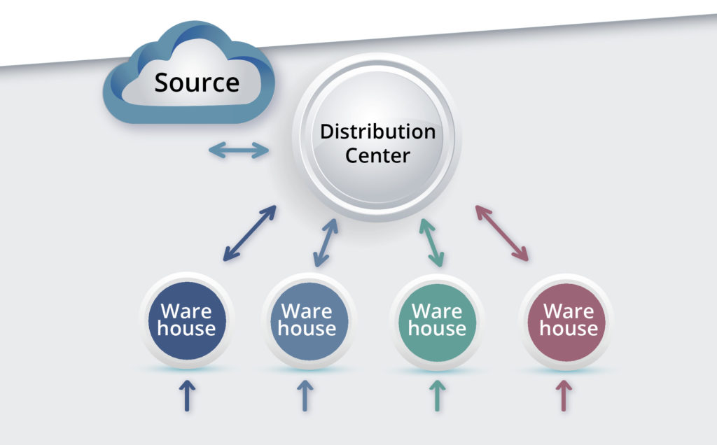
Figure 1: General structure of one type of two-level inventory system
Imagine the higher level to consist of a single distribution center (DC) which does not service customers directly but does replenish the WHs. For simplicity, assume the DC itself is replenished from a Source that always has (or makes) sufficient stock to immediately ship parts to the DC, though with some delay. (Alternatively, we could consider the system to have retail stores supplied by one warehouse).
Each level can be described in terms of demand levels (treated as random), lead times (random), inventory control parameters (here, Min and Max values) and shortage policy (here, backorders allowed).
The Method of Analysis
The academic literature has made progress on this problem, though usually at the cost of simplifications necessary to facilitate a purely mathematical solution. Our approach here is more accessible and flexible: Monte Carlo simulation. That is, we build a computer program that incorporates the logic of the system operation. The program “creates” random demand at the WH level, processes the demand according to the logic of a chosen inventory policy, and creates demand for the DC by pooling the random requests for replenishment made by the WHs. This approach lets us observe many simulated days of system operation while watching for significant events like stockouts at either level.
An Example
To illustrate an analysis, we simulated a system consisting of four WHs and one DC. Average demand varied across the WHs. Replenishment from the DC to any WH took from 4 to 7 days, averaging 5.15 days. Replenishment of the DC from the Source took either 7, 14, 21 or 28 days, but 90% of the time it was either 21 or 28 days, making the average 21 days. Each facility had Min and Max values set by analyst judgement after some rough calculations.
Figure 2 shows the results of one year of simulated daily operation of this system. The first row in the figure shows the daily demand for the item at each WH, which was assumed to be “purely random”, meaning it had a Poisson distribution. The second row shows the on-hand inventory at the end of each day, with Min and Max values indicated by blue lines. The third row describes operations at the DC. Contrary to the assumption of much theory, the demand into the DC was not close to being Poisson, nor was the demand out of the DC to the Source. In this scenario, Min and Max values were sufficient to keep item availability was high at each WH and at the DC, with no stockouts observed at any of the five facilities.
Click here to enlarge the image
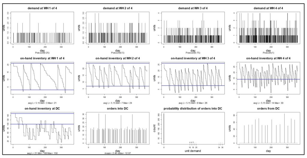
Figure 2 – Simulated year of operation of a system with four WHs and one DC.
Now let’s vary the scenario. When stockouts are extremely rare, as in Figure 2, there is often excess inventory in the system. Suppose somebody suggests that the inventory level at the DC looks a bit fat and thinks it would be good idea to save money there. Their suggestion for reducing the stock at the DC is to reduce the value of the Min at the DC from 100 to 50. What happens? You could guess, or you could simulate.
Figure 3 shows the simulation – the result is not pretty. The system runs fine for much of the year, then the DC runs out of stock and cannot catch up despite sending successively larger replenishment orders to the Source. Three of the four WHs descend into death spirals by the end of the year (and WH1 follows thereafter). The simulation has highlighted a sensitivity that cannot be ignored and has flagged a bad decision.
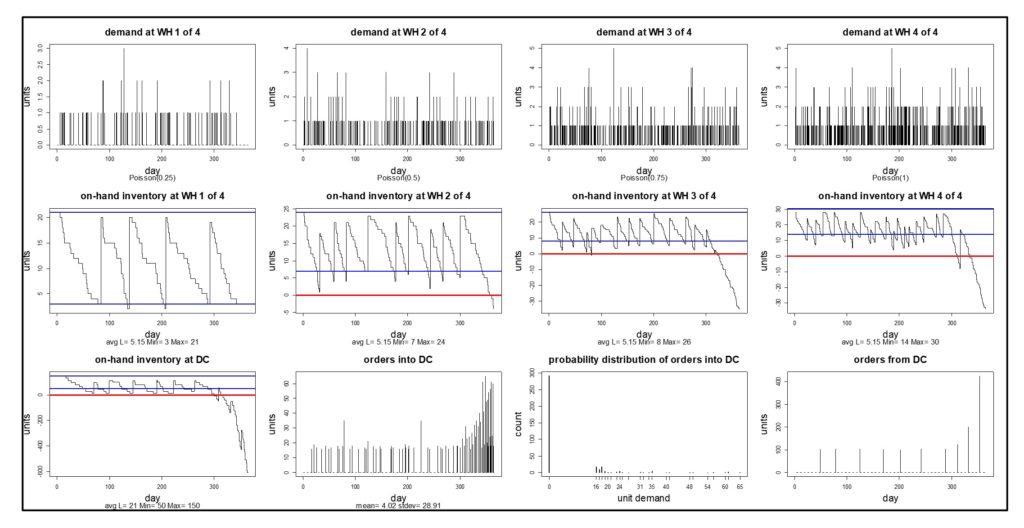
Figure 3 – Simulated effects of reducing the Min at the DC.
Now the inventory managers can go back to the drawing board and test out other possible ways to reduce the investment in inventory at the DC level. One move that always helps, if you and your supplier can jointly make it happen, is to create a more agile system by reducing replenishment lead time. Working with the Source to insure that the DC always gets its replenishments in either 7 or 14 days stabilizes the system, as shown in Figure 4.
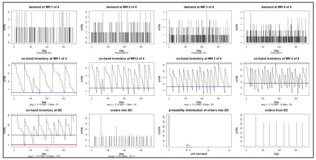
Figure 4 – Simulated effects of reducing the lead time for replenishing the DC.
Unfortunately, the intent of reducing the inventory at the DC has not been achieved. The original daily inventory count was about 80 units and remains about 80 units after reducing the DC’s Min and drastically improving the Source-to-DC lead time. But with the simulation model, the planning team can try out other ideas until they arrive at a satisfactory redesign. Or, given that Figure 4 shows the DC inventory starting to flirt with zero, they might think it prudent to accept the need for an average of about 80 units at the DC and look for ways to trim inventory investment at the WHs instead.
The Takeaways
- Multiechelon inventory optimization (MEIO) is complex. Many factors interact to produce system behaviors that can be surprising in even simple two-level systems.
- Monte Carlo simulation is a useful tool for planners who need to design new systems or tweak existing systems.


Managing Spare Parts Inventory: Best Practices
In this blog, we’ll explore several effective strategies for managing spare parts inventory, emphasizing the importance of optimizing stock levels, maintaining service levels, and using smart tools to aid in decision-making. Managing spare parts inventory is a critical component for businesses that depend on equipment uptime and service reliability. Unlike regular inventory items, spare parts often have unpredictable demand patterns, making them more challenging to manage effectively. An efficient spare parts inventory management system helps prevent stockouts that can lead to operational downtime and costly delays while also avoiding overstocking that unnecessarily ties up capital and increases holding costs.
12 Causes of Overstocking and Practical Solutions
Managing inventory effectively is critical for maintaining a healthy balance sheet and ensuring that resources are optimally allocated. Here is an in-depth exploration of the main causes of overstocking, their implications, and possible solutions.

FAQ: Mastering Smart IP&O for Better Inventory Management.
Effective supply chain and inventory management are essential for achieving operational efficiency and customer satisfaction. This blog provides clear and concise answers to some basic and other common questions from our Smart IP&O customers, offering practical insights to overcome typical challenges and enhance your inventory management practices. Focusing on these key areas, we help you transform complex inventory issues into strategic, manageable actions that reduce costs and improve overall performance with Smart IP&O.