Just as the renowned astronomer Copernicus transformed our understanding of astronomy by placing the sun at the center of our universe, today, we invite you to re-center your approach to inventory management. And while not quite as enlightening, this advice will help your company avoid being caught in the gravitational pull of inventory woes—constantly orbiting between stockouts, surplus gravity, and the unexpected cosmic expenses of expediting?

In this article, we’ll walk you through the process of crafting a spare parts inventory plan that prioritizes availability metrics such as service levels and fill rates while ensuring cost efficiency. We’ll focus on an approach to inventory planning called Service Level-Driven Inventory Optimization. Next, we’ll discuss how to determine what parts you should include in your inventory and those that might not be necessary. Lastly, we’ll explore ways to enhance your service-level-driven inventory plan consistently.

In service-oriented businesses, the consequences of stockouts are often very significant.  Achieving high service levels depends on having the right parts at the right time. However, having the right parts isn’t the only factor. Your Supply Chain Team must develop a consensus inventory plan for every part, then continuously update it to reflect real-time changes in demand, supply, and financial priorities.

Managing inventory with Service-level-driven planning combines the ability to plan thousands of items with high-level strategic modeling. This requires addressing core issues facing inventory executives:

• Lack of control over supply and associated lead times.
• Unpredictable intermittent demand.
• Conflicting priorities between maintenance/mechanical teams and Materials Management.
• Reactive “wait and see” approach to planning.
• Misallocated inventory, causing stockouts and excess.
• Lack of trust in systems and processes.

The key to optimal service parts management is to grasp the balance between providing excellent service and controlling costs. To do this, we must compare the costs of stockout with the cost of carrying additional spare parts inventory. The costs of a stockout will be higher for critical or emergency spares, when there is a service level agreement with external customers, for parts used in multiple assets, for parts with longer supplier lead times, and for parts with a single supplier. The cost of inventory may be assessed by considering the unit costs, interest rates, warehouse space that will be consumed, and potential for obsolescence (parts used on a soon-to-be-retired fleet have a higher obsolescence risk, for example).

To arbitrate how much stock should be put on the shelf for each part, it is critical to establish consensus on the desired key metrics that expose the tradeoffs the business must make to achieve the desired KPIs. These KPIs will include Service Levels that tell you how often you meet usage needs without falling short on stock, Fill Rates that tell you what percentage of demand is filled, and Ordering costs detail the expenses incurred when you place and receive replenishment orders. You also have Holding costs, which encompass expenses like obsolescence, taxes, and warehousing, and Shortage costs that pertain to expenses incurred when stockouts happen.

An MRO business or Aftermarket Parts Planning team might desire a 99% service level across all parts – i.e., the minimum stockout risk that they are willing to accept is 1%. But what if the amount of inventory needed to support that service level is too expensive? To make an informed decision on whether there is going to be a return on that additional inventory investment, you’ll need to know the stockout costs and compare that to the inventory costs. To get stockout costs, multiply two key elements: the cost per stockout and the projected number of stockouts. To get inventory value, multiply the units required by the unit cost of each part. Then determine the annual holding costs (typically 25-35% of the unit cost). Choose the option that yields a total lower cost. In other words, if the benefit associated with adding more stock (reduced shortage costs) outweighs the cost (higher inventory holding costs), then go for it. A thorough understanding of these metrics and the associated tradeoffs serves as the compass for decision-making.

Modern software aids in this process by allowing you to simulate a multitude of future scenarios. By doing so, you can assess how well your current inventory stocking strategies are likely to perform in the face of different demand and supply patterns. If anything falls short or goes awry, it’s time to recalibrate your approach, factoring in current data on usage history, supplier lead times, and costs to prevent both stockouts and overstock situations.

Enhance your service-level-driven inventory plan consistently.

In conclusion, it’s crucial to assess your service-level-driven plan continuously. By systematically constructing and refining performance scenarios, you can define key metrics and goals, benchmark expected performance, and automate the calculation of stocking policies for all items. This iterative process involves monitoring, revising, and repeating each planning cycle.

The depth of your analysis within these stocking policies relies on the data at your disposal and the configuration capabilities of your planning system. To achieve optimal outcomes, it’s imperative to maintain ongoing data analysis. This implies that a manual approach to data examination is typically insufficient for the needs of most organizations.

For information on how Smart Software can help you meet your service supply chain goals with service-driven planning and more, visit the following blogs.

–   “Explaining What  Service-Level Means in Your Inventory Optimization Software”  Stocking recommendations can be puzzling, especially when they clash with real-world needs.  In this post, we’ll break down what that 99% service level means and why it’s crucial for managing inventory effectively and keeping customers satisfied in today’s competitive landscape.

–  “Service-Level-Driven Planning for Service Parts Businesses” Service-Level-Driven Service Parts Planning is a four-step process that extends beyond simplified forecasting and rule-of-thumb safety stocks. It provides service parts planners with data-driven, risk-adjusted decision support.

–   “How to Choose a Target Service Level.” This is a strategic decision about inventory risk management, considering current service levels and fill rates, replenishment lead times, and trade-offs between capital, stocking and opportunity costs.  Learn approaches that can help.

–   “The Right Forecast Accuracy Metric for Inventory Planning.”  Just because you set a service level target doesn’t mean you’ll actually achieve it. If you are interested in optimizing stock levels, focus on the accuracy of the service level projection. Learn how.

In this Videoblog, we will explain how time series forecasting has emerged as a pivotal tool, particularly at the daily level, which Smart Software has been pioneering since its inception over forty years ago. The evolution of business practices from annual to more refined temporal increments like monthly and now daily data analysis illustrates a significant shift in operational strategies.

Initially, during the 1980s, the usual practice of using annual data for forecasting and the introduction of monthly data was considered innovative. This period marked the beginning of a trend toward increasing the resolution of data analysis, enabling businesses to capture and react to faster shifts in market dynamics. As we progressed into the 2000s, the norm of monthly data analysis was well-established, but the ‘cool kids’—innovators at the edge of business analytics—began experimenting with weekly data. This shift was driven by the need to synchronize business operations with increasingly volatile market conditions and consumer behaviors that demanded more rapid responses than monthly cycles could provide. Today, in the 2020s, while monthly data analysis remains common, the frontier has shifted again, this time towards daily data analysis, with some pioneers even venturing into hourly analytics.

The real power of daily data analysis lies in its ability to provide a detailed view of business operations, capturing daily fluctuations that might be overlooked by monthly or weekly data.  However, the complexities of daily data necessitate advanced analytical approaches to extract meaningful insights. At this level, understanding demand requires grappling with concepts like intermittency, seasonality, trend, and volatility. Intermittency, or the occurrence of zero-demand days, becomes more pronounced at a daily granularity and demands specialized forecasting techniques like Croston’s method for accurate predictions. Seasonality at a daily level can reveal multiple patterns—such as increased sales on weekends or holidays—that monthly data would mask. Trends can be observed as short-term increases or decreases in demand, demanding agile adjustment strategies. Finally, volatility at the daily level is accentuated, showing more significant swings in demand than seen in monthly or weekly analyses, which can affect inventory management strategies and the need for buffer stock. This level of complexity underscores the need for sophisticated analytical tools and expertise in daily data analysis.

In conclusion, the evolution from less frequent to daily time series forecasting marks a substantial shift in how businesses approach data analysis. This transition not only reflects the accelerating pace of business but also highlights the requirement for tools that can handle increased data granularity. Smart Software’s dedication to refining its analytical capabilities to manage daily data highlights the industry’s broader move towards more dynamic, responsive, and data-driven decision-making. This shift is not merely about keeping pace with time but about leveraging detailed insights to forge competitive advantages in an ever-changing business environment.

​

​Demand planning and statistical forecasting software play a pivotal role in effective business management by incorporating features that significantly enhance forecasting accuracy. One key aspect involves the utilization of smoothing-based or extrapolative models, enabling businesses to quickly make predictions based solely on historical data. This foundation rooted in past performance is crucial for understanding trends and patterns, especially in variables like sales or product demand. Forecasting software goes beyond mere data analysis by allowing the blending of professional judgment with statistical forecasts, recognizing that forecasting is not a one-size-fits-all process. This flexibility enables businesses to incorporate human insights and industry knowledge into the forecasting model, ensuring a more nuanced and accurate prediction.

Features such as forecasting multiple items as a group, considering promotion-driven demand, and handling intermittent demand patterns are essential capabilities for businesses dealing with diverse product portfolios and dynamic market conditions.  Proper implementation of these applications empowers businesses with versatile forecasting tools, contributing significantly to informed decision-making and operational efficiency.

Extrapolative models

Our demand forecasting solutions support a variety of forecasting approaches including extrapolative or smoothing-based forecasting models, such as exponential smoothing and moving averages.  The philosophy behind these models is simple: they try to detect, quantify, and project into the future any repeating patterns in the historical data.

  There are two types of patterns that might be found in the historical data:

• Trend
• Seasonality

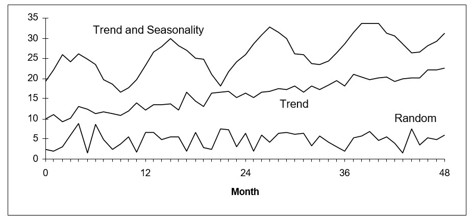
These patterns are illustrated in the following figure along with random data.

Illustrating trending, seasonal, and random time series data

If the pattern is a trend, then extrapolative models such as double exponential smoothing and linear moving average estimates the rate of increase or decrease in the level of the variable and project that rate into the future.

If the pattern is seasonality, then models such as Winters and triple exponential smoothing estimate either seasonal multipliers or seasonal add factors and then apply these to projections of the nonseasonal portion of the data.

Very often, especially with retail sales data, both trend and seasonal patterns are involved. If these patterns are stable, they can be exploited to give very accurate forecasts.

Sometimes, however, there are no obvious patterns, so that plots of the data look like random noise. Sometimes patterns are clearly visible, but they change over time and cannot be relied upon to repeat. In these cases, the extrapolative models don’t try to quantify and project patterns. Instead, they try to average through the noise and make good estimates of the middle of the distribution of data values. These typical values then become the forecasts.  Sometimes, when users see a historical plot with lots of ups and downs they are concerned when the forecast doesn’t replicate those ups and downs. Normally, this should not be a reason for concern.  This occurs when the historical patterns aren’t strong enough to warrant using a forecasting method that would replicate the pattern.  You want to make sure your forecasts don’t suffer from the “wiggle effect” that is described in this blog post.

Past as a predictor of the future

The key assumption implicit in extrapolative models is that the past is a good guide to the future. This assumption, however, can break down. Some of the historical data may be obsolete. For example, the data might describe a business environment that no longer exists. Or, the world that the model represents may be ready to change soon, rendering all the data obsolete. Because of such complicating factors, the risks of extrapolative forecasting are lower when forecasting only a short time into the future.

Extrapolative models have the practical advantage of being cheap and easy to build, maintain and use. They require only accurate records of past values of the variables you need to forecast. As time goes by, you simply add the latest data points to the time series and reforecast. In contrast, the causal models described below require more thinking and more data. The simplicity of extrapolative models is most appreciated when you have a massive forecasting problem, such as making overnight forecasts of demand for all 30,000 items in inventory in a warehouse.

Judgmental adjustments

Extrapolative models can be run in a fully automatic mode with Demand Planner with no intervention required. Causal models require substantive judgment for wise selection of independent variables. However, both types of statistical models can be enhanced by judgmental adjustments. Both can profit from your insights.

Both causal and extrapolative models are built on historical data. However, you may have additional information that is not reflected in the numbers found in the historical record. For instance, you may know that competitive conditions will soon change, perhaps due to price discounts, or industry trends, or the emergence of new competitors, or the announcement of a new generation of your own products. If these events occur during the period for which you are forecasting, they may well spoil the accuracy of purely statistical forecasts. Smart Demand Planner’ graphical adjustment feature lets you include these additional factors in your forecasts through the process of on- screen graphical adjustment.

Be aware that applying user adjustments to the forecast is a two-edged sword. Used appropriately, it can enhance forecast accuracy by exploiting a richer set of information. Used promiscuously, it can add additional noise to the process and reduce accuracy. We advise that you use judgmental adjustments sparingly, but that you never blindly accept the predictions of a purely statistical forecasting method.  It is also very important to measure forecast value add.  That is, the value added to the forecast process by each incremental step.  For example, if you are applying overrides based on business knowledge, it is important to measure whether those adjustments are adding value by improving forecast accuracy.  Smart Demand Planner supports measurement of forecast value add by tracking every forecast considered and automating the forecast accuracy reports. You can select statistical forecasts, measure their errors, and compare them to the overridden ones.  By doing so, you inform the forecasting process so that better decisions can be made in the future. 

Multiple-level forecasts

Another common situation involves multiple-level forecasting, where there are multiple items being forecast as a group or there may even be multiple groups, with each group containing multiple items. We will generally call this type of forecasting Multilevel Forecasting. The prime example is product line forecasting, where each item is a member of a family of items, and the total of all the items in the family is a meaningful quantity.

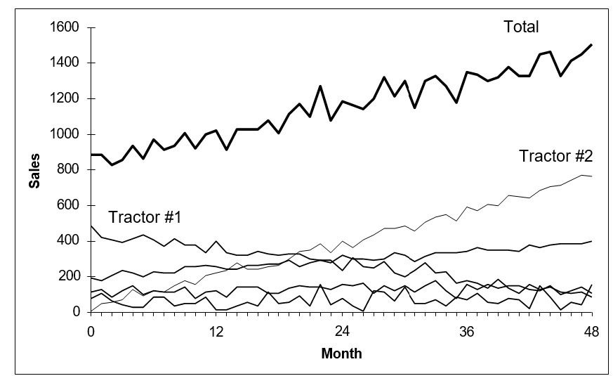
For example, as in the following figure, you might have a line of tractors and want forecasts of sales for each type of tractor and for the entire tractor line.

Illustrating multiple-level product forecasts

 Smart Demand Planner provides Roll Up/Roll Down Forecasting. This function is crucial for obtaining comprehensive forecasts of all product items and their group total. The Roll Down/Roll Up method within this feature offers two options for obtaining these forecasts:

Roll Up (Bottom-Up): This option initially forecasts each item individually and then aggregates the item-level forecasts to generate a family-level forecast.

Roll Down (Top-Down): Alternatively, the roll-down option starts by forming the historical total at the family level, forecasts it, and then proportionally allocates the total down to the item level.

When utilizing Roll Down/Roll Up, you have access to the full array of forecast methods provided by Smart Demand Planner at both the item and family levels. This ensures flexibility and accuracy in forecasting, catering to the specific needs of your business across different hierarchical levels.

Forecasting research has not established clear conditions favoring either the top-down or bottom-up approach to forecasting. However, the bottom-up approach seems preferable when item histories are stable, and the emphasis is on the trends and seasonal patterns of the individual items. Top-down is normally a better choice if some items have very noisy history or the emphasis is on forecasting at the group level. Since Smart Demand Planner makes it fast and easy to try both a bottom-up and a top- down approach, you should try both methods and compare the results.  You can use Smart Demand Planner’s “Hold back on Current”  feature in the “Forecast vs. Actual” to test both approaches on your own data and see which one yields a more accurate forecast for your business. 

In this video blog, we explore the integral role that inventory models play in shaping the decision-making processes of professionals across various industries. These models, whether they are tangible computer simulations or intangible mental constructs, serve as critical tools in managing the complexities of modern business environments. The discussion begins with an overview of how these models are utilized to predict outcomes and streamline operations, emphasizing their relevance in a constantly evolving market landscape.

​The discussion further explores how various models distinctly influence strategic decision-making processes. For instance, the mental models professionals develop through experience often guide initial responses to operational challenges. These models are subjective, built from personal insights and past encounters with similar situations, allowing quick, intuitive decision-making. On the other hand, computer-based models provide a more objective framework. They use historical data and algorithmic calculations to forecast future scenarios, offering a quantitative basis for decisions that need to consider multiple variables and potential outcomes. This section highlights specific examples, such as the impact of adjusting order quantities on inventory costs and ordering frequency or the effects of fluctuating lead times on service levels and customer satisfaction.

In conclusion, while mental models provide a framework based on experience and intuition, computer models offer a more detailed and numbers-driven perspective. Combining both types of models allows for a more robust decision-making process, balancing theoretical knowledge with practical experience. This approach enhances the understanding of inventory dynamics and equips professionals with the tools to adapt to changes effectively, ensuring sustainability and competitiveness in their respective fields.

For some of our customers, weather has a significant influence on demand. Extreme short-term weather events like fires, droughts, hot spells, and so forth can have a significant near-term influence on demand.

There are two ways to factor weather into a demand forecast: indirectly and directly. The indirect route is easier using the scenario-based approach of Smart Demand Planner. The direct approach requires a tailored special project requiring additional data and hand-crafted modeling.

Indirect Accounting for Weather

The standard model built into Smart Demand Planner (SDP) accommodates weather effects in four ways:

1. If the world is steadily getting warmer/colder/drier/wetter in ways that impact your sales, SDP detects these trends automatically and incorporates them into the demand scenarios it generates.
2. If your business has a regular rhythm in which certain days of the week or certain months of the year have consistently higher or lower-than-average demand, SDP also automatically detects this seasonality and incorporates it into its demand scenarios.
3. Often it is the cussed randomness of weather that interferes with forecast accuracy. We often refer to this effect as “noise”. Noise is a catch-all term that incorporates all kinds of random trouble. Besides weather, a geopolitical flareup, the surprise failure of a regional bank, or a ship getting stuck in the Suez Canal can and have added surprises to product demand. SDP assesses the volatility of demand and reproduces it in its demand scenarios.
4. Management overrides. Most of the time, customers let SDP churn away to automatically generate tens of thousands of demand scenarios. But if users feel the need to touch up specific forecasts using their insider knowledge, SDP can make that happen through management overrides.

Direct Accounting for Weather

Sometimes a user will be able to articulate subject matter expertise linking factors outside their company (such as interest rates or raw materials costs or technology trends) to their own aggregate sales. In these situations, Smart Software can arrange for one-off special projects that provide alternative (“causal”) models to supplement our standard statistical forecasting models. Contact your Smart Software representative to discuss a possible causal modeling project.

Meanwhile, don’t forget your umbrella.