Are you confused about what is AI and what is machine learning? Are you unsure why knowing more will help you with your job in inventory planning? Don’t despair. You’ll be ok, and we’ll show you how some of whatever-it-is can be useful.

What is and what isn’t

What is AI and how does it differ from ML? Well, what does anybody do these days when they want to know something? They Google it. And when they do, the confusion starts.

One source says that the neural net methodology called deep learning is a subset of machine learning, which is a subset of AI. But another source says that deep learning is already a part of AI because it sort of mimics the way the human mind works, while machine learning doesn’t try to do that.

One source says there are two types of machine learning: supervised and unsupervised. Another says there are four: supervised, unsupervised, semi-supervised and reinforcement.

Some say reinforcement learning is machine learning; others call it AI.

Some of us traditionalists call a lot of it “statistics”, though not all of it is.

In the naming of methods, there is a lot of room for both emotion and salesmanship. If a software vendor thinks you want to hear the phrase “AI”, they may well say it for you just to make you happy.

Better to focus on what comes out at the end

You can avoid some confusing hype if you focus on the end result you get from some analytic technology, regardless of its label. There are several analytical tasks that are relevant to inventory planners and demand planners. These include clustering, anomaly detection, regime change detection, and regression analysis. All four methods are usually, but not always, classified as machine learning methods. But their algorithms can come straight out of classical statistics.

Clustering

Clustering means grouping together things that are similar and distancing them from things that are dissimilar. Sometimes clustering is easy: to separate your customers geographically, simply sort them by state or sales region. When the problem is not so dead obvious, you can use data and clustering algorithms to get the job done automatically even when dealing with massive datasets.

For example, Figure 1 illustrates a cluster of “demand profiles”, which in this case divides all a customer’s items into nine clusters based on the shape of their cumulative demand curves. Cluster 1.1 in the top left contains items whose demand has been petering out, while Cluster 3.1 in the bottom left contains items whose demand has accelerated.  Clustering can also be done on suppliers. The choice of number of clusters is typically left to user judgement, but ML can guide that choice.  For example, a user might instruct the software to “break my parts into 4 clusters” but using ML may reveal that there are really 6 distinct clusters the user should analyze. 

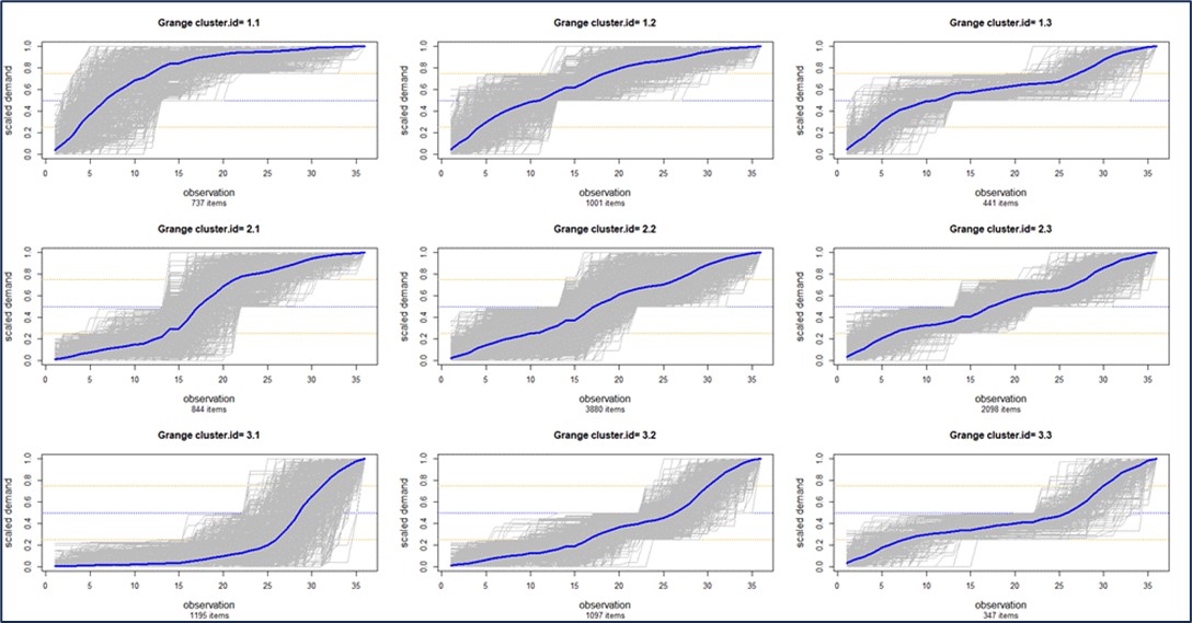
Figure 1: Clustering items based on the shapes of their cumulative demand

Anomaly Detection

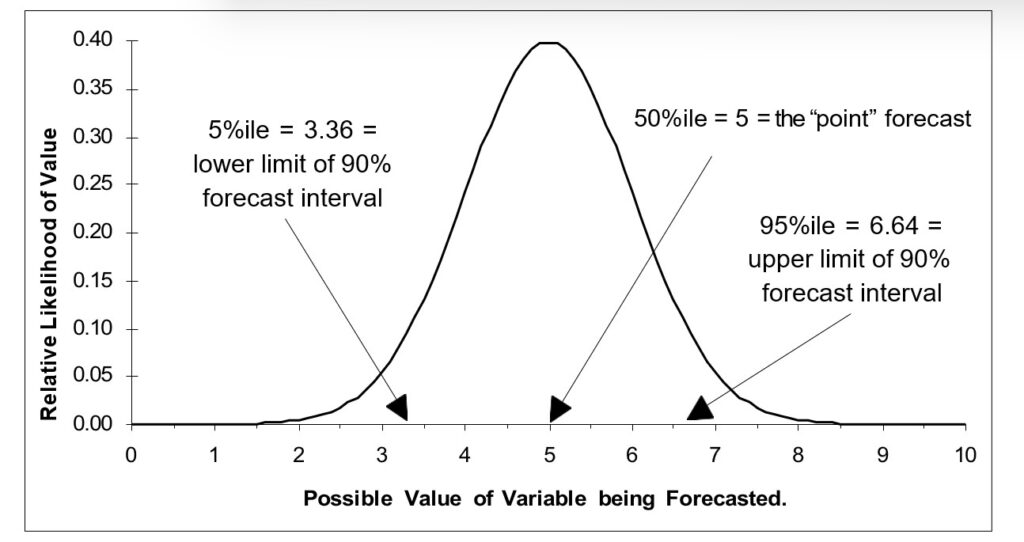
Demand forecasting is traditionally done using time series extrapolation. For instance, simple exponential smoothing works to find the “middle” of the demand distribution at any time and project that level forward. However, if there has been a sudden, one-time jump up or down in demand in the recent past, that anomalous value can have a significant but unwelcome effect on the near-term forecast.  Just as serious for inventory planning, the anomaly can have an outsized effect on the estimate of demand variability, which goes directly to the calculation of safety stock requirements.

Planners may prefer to find and remove such anomalies (and maybe do offline follow-up to find out the reason for the weirdness). But nobody with a big job to do will want to visually scan thousands of demand plots to spot outliers, expunge them from the demand history, then recalculate everything. Human intelligence could do that, but human patience would soon fail. Anomaly detection algorithms could do the work automatically using relatively straightforward statistical methods. You could call this “artificial intelligence” if you wish.

Regime Change Detection

Regime change detection is like the big brother of anomaly detection. Regime change is a sustained, rather than temporary, shift in one or more aspects of the character of a time series. While anomaly detection usually focuses on sudden shifts in mean demand, regime change could involve shifts in other features of the demand, such as its volatility or its distributional shape.  

Figure 2 illustrates an extreme example of regime change. The bottom dropped out of demand for this item around day 120. Inventory control policies and demand forecasts based on the older data would be wildly off base at the end of the demand history.

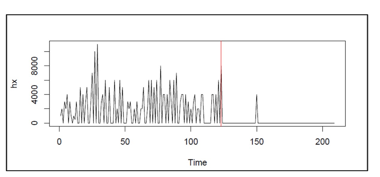
Figure 2: An example of extreme regime change in an item with intermittent demand

Here too, statistical algorithms can be developed to solve this problem, and it would be fair play to call them “machine learning” or “artificial intelligence” if so motivated.  Using ML or AI to identify regime changes in demand history enables demand planning software to automatically use only the relevant history when forecasting instead of having to manually pick the amount of history to introduce to the model. 

Regression analysis

Regression analysis relates one variable to another through an equation. For example, sales of window frames in one month may be predicted from building permits issued a few months earlier. Regression analysis has been considered a part of statistics for over a century, but we can say it is “machine learning” since an algorithm works out the precise way to convert knowledge of one variable into a prediction of the value of another.

Summary

It is reasonable to be interested in what’s going on in the areas of machine learning and artificial intelligence. While the attention given to ChatGPT and its competitors is interesting, it is not relevant to the numerical side of demand planning or inventory management. The numerical aspects of ML and AI are potentially relevant, but you should try to see through the cloud of hype surrounding these methods and focus on what they can do.  If you can get the job done with classical statistical methods, you might just do that, then exercise your option to stick the ML label on anything that moves.

Forecasting inventory requirements is a specialized variant of forecasting that focuses on the high end of the range of possible future demand.

For simplicity, consider the problem of forecasting inventory requirements for just one period ahead, say one day ahead. Usually, the forecasting job is to estimate the most likely or average level of product demand. However, if available inventory equals the average demand, there is about a 50% chance that demand will exceed inventory and result in lost sales and/or lost good will. Setting the inventory level at, say, ten times the average demand will probably eliminate the problem of stockouts, but will just as surely result in bloated inventory costs.

The trick of inventory optimization is to find a satisfactory balance between having enough inventory to meet most demand without tying up too many resources in the process. Usually, the solution is a blend of business judgment and statistics. The judgmental part is to define an acceptable inventory service level, such as meeting 95% of demand immediately from stock. The statistical part is to estimate the 95th percentile of demand.

When not dealing with intermittent demand, you can often estimate the required inventory level by assuming a bell-shaped (Normal) curve of demand, estimating both the middle and the width of the bell curve, then using a standard statistical formula to estimate the desired percentile. The difference between the desired inventory level and the average level of demand is called the “safety stock” because it protects against the possibility of stockouts.

When dealing with intermittent demand, the bell-shaped curve is a very poor approximation to the statistical distribution of demand. In this special case, Smart leverages patented technology for intermittent demand that is designed to accurately forecast the ranges and produce a better estimate of the safety stock needed to achieve the required inventory service level.

Every field, including forecasting, accumulates folk wisdom that eventually starts masquerading as “best practices.”  These best practices are often wise, at least in part, but they often lack context and may not be appropriate for certain customers, industries, or business situations.  There is often a catch, a “Yes, but”. This note is about six usually true forecasting precepts that nevertheless do have their caveats.

1. Organize your company around a one-number forecast. This sounds sensible: it’s good to have a shared vision. But each part of the company will have its own idea about which number is the number. Finance may want quarterly revenue, Marketing may want web site visits, Sales may want churn, Maintenance may want mean time to failure. For that matter, each unit probably has a handful of key metrics. You don’t need a slogan – you need to get your job done.

2. Incorporate business knowledge into a collaborative forecasting process. This is a good general rule, but if your collaborative process is flawed, messing with a statistical forecast via management overrides can decrease accuracy. You don’t need a slogan – you need to measure and compare the accuracy of any and all methods and go with the winners.

3. Forecast using causal modeling. Extrapolative forecasting methods take no account of the underlying forces driving your sales, they just work with the results. Causal modeling takes you deeper into the fundamental drivers and can improve both accuracy and insight. However, causal models (implemented through regression analysis) can be less accurate, especially when they require forecasts of the drivers (“predictions of the predictors”) rather than simply plugging in recorded values of lagged predictor variables. You don’t need a slogan: You need a head-to-head comparison.

4. Forecast demand instead of shipments. Demand is what you really want, but “composing a demand signal” can be tricky: what do you do with internal transfers? One-off’s?  Lost sales? Furthermore, demand data can be manipulated.  For example, if customers intentionally don’t place orders or try to game their orders by ordering too far in advance, then order history won’t be better than shipment history.  At least with shipment history, it’s accurate:  You know what you shipped. Forecasts of shipments are not forecasts of  “demand”, but they are a solid starting point.

5. Use Machine Learning methods. First, “Machine learning” is an elastic concept that includes an ever-growing set of alternatives. Under the hood of many ML advertised models is just an auto-pick an extrapolative forecast method (i.e., best fit) which while great at forecasting normal demand, has been around since the 1980’s (Smart Software was the first company to release an auto-pick method for the PC).   ML models are data hogs that require larger data sets than you may have available. Properly choosing then training an ML model requires a level of statistical expertise that is uncommon in many manufacturing and distribution businesses. You might want to find somebody to hold your hand before you start playing this game.

6. Removing outliers creates better forecasts. While it is true that very unusual spikes or drops in demand will mask underlying demand patterns such as trend or seasonality, it isn’t always true that you should remove the spikes. Often these demand surges reflect the uncertainty that can randomly interfere with your business and thus need to be accounted for.  Removing this type of data from your demand forecast model might make the data more predictable on paper but will leave you surprised when it happens again. So, be careful about removing outliers, especially en masse.

Customers often ask us why a stocking recommendation is “so high.” Here is a question we received recently:

During our last team meeting, we found a few items with abnormal gaps between our current ROP and the Smart-suggested ROP at a 99% service level. The concern is that the system indicates that the reorder point will have to increase substantially to achieve a 99% service level. Would you please help us understand the calculation?

When we reviewed the data, it was clear to the customer that the Smart-calculated ROP was indeed correct.  We concluded (1) what they really wanted was a much lower service level target and (2) we had not done a good explaining what was really meant by “service level.” 

So, what does a “99% service level” really mean? 

When it pertains to the target that you enter in your inventory optimization software, it means that the stocking level for the item in question will have a 99% chance of being able to fill whatever the customer needs right away.  For instance, if you have 50 units in stock, there is a 99% chance that the next demand will fall somewhere in the range of 0 to 50 units.

What our customer meant was that 99% of the time a customer placed an order, it was delivered in full within whatever lead time the customer was quoted.  In other words, not necessarily right away but when promised.  

Obviously, the more time you give yourself to deliver to a customer the higher your service level will be. But that distinction is often not explicitly understood when new users of inventory optimization software are conducting what-if scenarios at different service levels.  And that can lead to considerable confusion.  Computing service levels based on immediate stock availability is a higher standard: harder to meet but much more competitive.

Our manufacturing customers often quote service levels based on lead times to their customers, so it isn’t essential for them to deliver immediately from the shelf. In contrast, our customers in the distribution, Maintenance Repair and Operations (MRO), and spare parts spaces, must normally ship same day or within 24 hours.  For them it is a competitive necessity to ship right away and do so in full.

When inputting target service levels using your inventory optimization software, keep this distinction in mind.  Choose the service level based on the percentage of the time you want to ship inventory in full, right away from the shelf.  

A forecast is a prediction about the value of a time series variable at some time in the future. For instance, one might want to estimate next month’s sales or demand for a product item. A time series is a sequence of numbers recorded at equally spaced time intervals; for example, unit sales recorded every month.

The objectives you pursue when you forecast depend on the nature of your job and your business. Every forecast is uncertain; in fact, there is a range of possible values for any variable you forecast. Values near the middle of this range have a higher likelihood of actually occurring, while values at the extremes of the range are less likely to occur. The following figure illustrates a typical distribution of forecast values.

Illustrating a forecast distribution of forecast values

Point forecasts

The most common use of forecasts is to estimate a sequence of numbers representing the most likely future values of the variable of interest. For instance, suppose you are developing a sales and marketing plan for your company. You may need to fill in 12 cells in a financial spreadsheet with estimates of your company’s total revenues over the next 12 months. Such estimates are called point forecasts because you want a single number (data point) for each forecast period. Smart Demand Planner’ Automatic forecasting feature provides you with these point forecasts automatically.

Interval forecasts

Although point forecasts are convenient, you will often benefit more from interval forecasts. Interval forecasts show the most likely range (interval) of values that might arise in the future. These are usually more useful than point forecasts because they convey the amount of uncertainty or risk involved in a forecast. The forecast interval percentage can be specified in the various forecasting dialog boxes in the Demand Planning Software.  Each of the many forecasting methods (automatic, moving average, exponential smoothing and so on) available in Smart Demand Planner allow you to set a forecast interval.

The default configuration in Smart Demand Planner provides 90% forecast intervals. Interpret these intervals as the range within which the actual values will fall 90% of the time. If the intervals are wide, then there is a great deal of uncertainty associated with the point forecasts. If the intervals are narrow, you can be more confident. If you are performing a planning function and want best case and worst case values for the variables of interest at several times in the future, you can use the upper and lower limits of the forecast intervals for that purpose, with the single point estimate providing the most likely value. In the previous figure, the 90% forecast interval extends from 3.36 to 6.64.

Upper percentiles

In inventory control, your goal may be to make good estimates of a high percentile of the demand for a product item. These estimates help you cope with the tradeoff between, on the one hand, minimizing the costs of holding and ordering stock, and, on the other hand, minimizing the number of lost or back-ordered sales due to a stock out. For this reason, you may wish to know the 99th percentile or service level of demand, since the chance of exceeding that level is only 1%.

When forecasting individual variables with features like Automatic forecasting, note that the upper limit of a 90% forecast interval represents the 95th percentile of the predicted distribution of the demand for that variable. (Subtracting the 5th percentile from the 95th percentile leaves an interval containing 95%-5% = 90% of the possible values.) This means you can estimate upper percentiles by changing the value of the forecast interval. In the figure, “Illustrating a forecast distribution”, the 95th percentile is 6.64.

To optimize stocking policies at the desired service level or to let the system recommend which stocking policy and service level generates the best return, consider using Smart Inventory Optimization.   It is designed to support what-if scenarios that show predicted tradeoffs of varying inventory polices including different service level targets.

Lower percentiles

Sometimes you may be concerned with the lower end of the predicted distribution for a variable. Such cases often arise in financial applications, where a low percentile of a revenue estimate represents a contingency requiring financial reserves. You can use Smart Demand Planner in this case in a way analogous to the case of forecasting upper percentiles. In the figure, “Illustrating a forecast distribution” , the 5th percentile is 3.36.

In conclusion, forecasting involves predicting future values, with point forecasts offering single estimates and interval forecasts providing likely value ranges. Smart Demand Planner automates point forecasts and allows users to set intervals, aiding in uncertainty assessment. For inventory control, the tool facilitates understanding upper (e.g., 99th percentile) and lower (e.g., 5th percentile) percentiles. To optimize stocking policies and service levels, Smart Inventory Optimization supports what-if scenarios, ensuring effective decision-making on how much to stock given the risk of stock out you are willing to accept.