Demand planning goes beyond simply forecasting product needs; it’s about ensuring your business meets customer demands with precision, efficiency, and cost-effectiveness. Latest demand planning technology addresses key challenges like forecast accuracy, inventory management, and market responsiveness. In this blog, we will introduce critical demand planning trends, including data-driven insights, probabilistic forecasting, consensus planning, predictive analytics, scenario modeling, real-time visibility, and multilevel forecasting. These trends will help you stay ahead of the curve, optimize your supply chain, reduce costs, and enhance customer satisfaction, positioning your business for long-term success.

Data-Driven Insights

Advanced analytics, machine learning, and artificial intelligence (AI) are becoming integral to demand planning. Technologies like Smart UP&O allow businesses to analyze complex data sets, identify patterns, and make more accurate predictions. This shift towards data-driven insights helps businesses respond quickly to market changes, minimizing stockouts and reducing excess inventory.

Probabilistic Forecasting

Probabilistic forecasting focuses on predicting a range of possible outcomes rather than a single figure. This trend is particularly important for managing uncertainty and risk in demand planning. It helps businesses prepare for various demand scenarios, enhancing inventory management and reducing the likelihood of stockouts or overstocking​.

Consensus Forecasting

Modern manufacturing is moving towards an integrated approach where departments and stakeholders collaborate more closely. Collaborative forecasting involves sharing insights across the supply chain, from suppliers to distributors and internal teams. This approach breaks down silos and ensures that everyone is working towards a common goal, leading to a more synchronized and efficient supply chain​.

Predictive and Prescriptive Analytics

Predictive analytics forecasts future outcomes based on historical data and trends, helping businesses anticipate demand fluctuations. For example, Smart Demand Planner (SDP) automates forecasting to adjust inventory and production levels accordingly​.

Prescriptive analytics goes further by offering actionable recommendations. Smart Inventory Planning and Optimization (IP&O), for instance, prescribes optimal inventory policies based on service levels, costs, and risks​. ogether, these tools enable proactive decision-making, allowing companies to both predict and optimize their responses to future challenges.

Scenario Modeling

Scenario modeling is becoming a key part of demand planning, enabling businesses to simulate different scenarios and assess their impact on operations. This method helps companies create adaptable strategies to effectively handle uncertainties. Smart IP&O enhances this capability by offering What If Scenarios that allow users to test different inventory policies before implementation. By adjusting variables like service levels or order quantities, businesses can visualize the effects on costs and service levels, empowering them to select the optimal strategy for minimizing risks and controlling costs​​.

Real-Time Visibility

As supply chains become more global and interconnected, real-time visibility into inventory and supply chain activities is crucial. Enhanced collaboration with suppliers and distributors, combined with real-time data, enables businesses to make quicker, more informed decisions. This helps optimize inventory levels, reduce lead times, and improve overall supply chain resilience​.

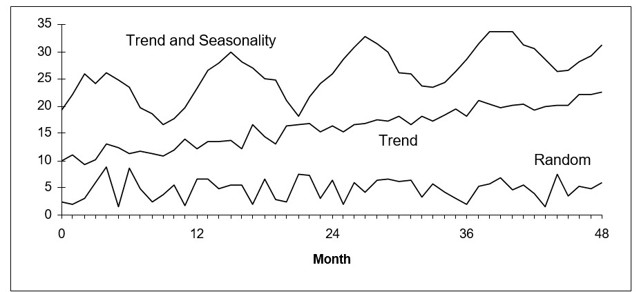
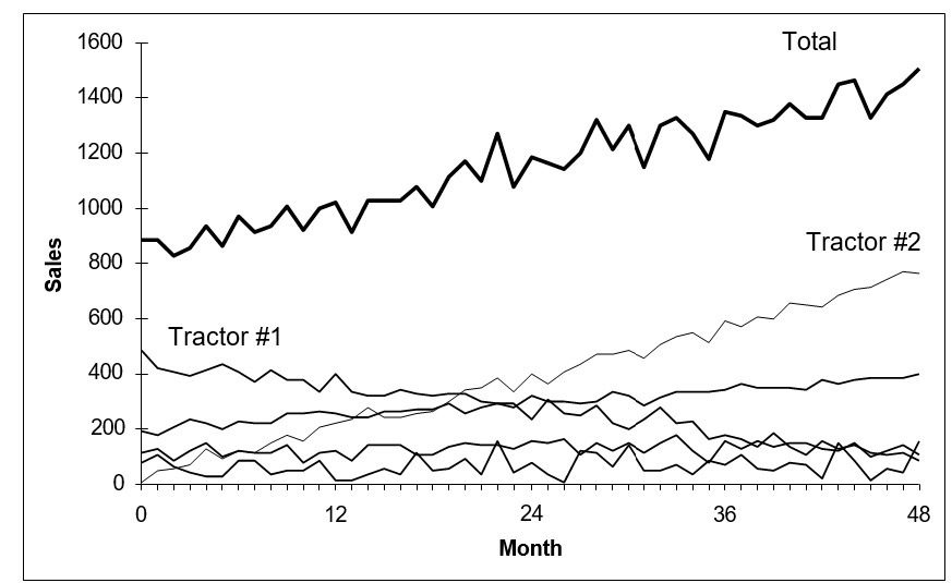
Multilevel Forecasting

This involves forecasting at different levels of the product hierarchy, such as individual items, product families, or even entire product lines. Multilevel forecasting is vital for businesses with complex product portfolios, as it ensures that forecasts are accurate at both the micro and macro levels​.

Demand planning is a decisive aspect of modern supply chain management, offering businesses the ability to enhance operational efficiency, reduce costs, and better meet customer demands. Leveraging advanced platforms like Smart IP&O significantly improves forecasting accuracy and inventory management, enabling swift responses to market fluctuations. Automated statistical forecasting, combined with capabilities like hierarchy forecasting and forecast overrides, ensures that forecasts are accurate and adaptable, leading to more realistic planning decisions. Additionally, with tools like scenario modeling, businesses can explore various demand scenarios across their product hierarchy, facilitating informed decision-making by providing insights into potential outcomes and risks. This approach allows businesses to anticipate the impact of policy changes, make better decisions, and ultimately optimize their inventory and overall supply chain management, staying ahead of key trends in the process.

In this blog, we will analyze the automatic forecasting for time series demand projections, focusing on key techniques, challenges, and best practices. There are multiple methods to predict future demand for an item, and this becomes complex when dealing with thousands of items, each requiring a different forecasting technique due to their unique demand patterns. Some items have stable demand, others trend upwards or downwards, and some exhibit seasonality. Selecting the right method for each item can be overwhelming. Here, we’ll explore how automatic forecasting simplifies this process.

Automatic forecasting becomes fundamental in managing large-scale demand projections. With thousands of items, manually selecting a forecasting method for each is impractical. Automatic forecasting uses software to make these decisions, ensuring accuracy and efficiency in the forecasting process. It’s importance lies in its ability to handle complex, large-scale forecasting needs efficiently. It eliminates the need for manual selection, saving time and reducing errors. This approach is particularly beneficial in environments with diverse demand patterns, where each item may require a different forecasting method.

Key Considerations for Effective Forecasting

1. Challenges of Manual Forecasting:
   • Infeasibility: Manually choosing forecasting methods for thousands of items is unmanageable.
   • Inconsistency: Human error can lead to inconsistent and inaccurate forecasts.
2. Criteria for Method Selection:
   • Error Measurement: The primary criterion for selecting a forecasting method is the typical forecast error, defined as the difference between predicted and actual values. This error is averaged over the forecast horizon (e.g., monthly forecasts over a year).
   • Holdout Analysis: This technique simulates the process of waiting for a year to elapse by hiding some historical data, making forecasts, and then revealing the hidden data to compute errors. This helps in choosing the best method in real-time.
3. Forecasting Tournament:
   • Method Comparison: Different methods compete to forecast each item, with the method producing the lowest average error winning.
   • Parameter Tuning: Each method is tested with various parameters to find the optimal settings. For example, simple exponential smoothing may be tried with different weighting factors.

The Algorithms Behind Effective Automatic Forecasting

Automatic forecasting is highly computational but feasible with modern technology. The process involves:

• Data Segmentation: Dividing historical data into segments helps manage and leverage different aspects of historical data for more accurate forecasting. For instance, for a product with seasonal demand, data might be segmented by seasons to capture season-specific trends and patterns. This segmentation allows forecasters to make and test forecasts more effectively.
• Repeated Simulations: Using sliding simulations involves repeatedly testing and refining forecasts over different periods. This method validates the accuracy of forecasting methods by applying them to different segments of data. An example is the sliding window method, where a fixed-size window moves across the time series data, generating forecasts for each position to evaluate performance.
• Parameter Optimization: Parameter optimization involves trying multiple variants of each forecasting method to find the best-performing one. By adjusting parameters, such as the smoothing factor in exponential smoothing methods or the number of past observations in ARIMA models, forecasters can fine-tune models to improve performance.

For instance, in our software, we allow various forecasting methods to compete for the best performance on a given item.  Knowledge of Automatic forecasting immediately carries over to Simple Moving Average, linear moving average, Single Exponential Smoothing, Double Exponential Smoothing, Winters’ Exponential Smoothing, and Promo forecasting. This competition ensures that the most suitable method is selected based on empirical evidence, not subjective judgment. The tournament winner is the closest method to predicting new data values from old. Accuracy is measured by average absolute error (that is, the average error, ignoring any minus signs). The average is computed over a set of forecasts, each using a portion of the data, in a process known as sliding simulation, which we have explained previously in a previous blog.

Methods used in Automatic forecasting

Normally, there are six extrapolative forecasting methods competing in the Automatic forecasting tournament:

• Simple moving average
• Linear moving average
• Single exponential smoothing
• Double exponential smoothing
• Additive version of Winters’ exponential smoothing
• Multiplicative version of Winters’ exponential smoothing

The latter two methods are appropriate for seasonal series; however, they are automatically excluded from the tournament if there are fewer than two full seasonal cycles of data (for example, fewer than 24 periods of monthly data or eight periods of quarterly data). These six classical, smoothing-based methods have proven themselves to be easy to understand, easy to compute and accurate. You can exclude any of these methods from the tournament if you have a preference for some of the competitors and not others.

Automatic forecasting for time series data is essential for managing large-scale demand projections efficiently and accurately. Businesses can achieve better forecast accuracy and streamline their planning processes by automating the selection of forecasting methods and utilizing techniques like holdout analysis and forecasting tournaments. Embracing these advanced forecasting techniques ensures that businesses stay ahead in dynamic market environments, making informed decisions based on reliable data projections.

In this blog, we are steering the conversation towards the transformative potential of technology in inventory management. The discussion centers around the limitations of simple thinking in managing inventory control processes and the necessity of adopting systematic software solutions. Dr. Tom Willemain highlights the contrast between Smart Software and the basic, albeit comfortable, approaches commonly employed by many businesses. These elementary methods, often favored for their ease of use and zero cost, are scrutinized for their inadequacies in addressing the dynamic challenges of inventory management.

​

​The importance of this subject lies in the critical role inventory management plays in a business’s operational efficiency and its direct impact on customer satisfaction and profitability. Dr. Tom Willemain points out the common pitfalls of relying on oversimplified rules of thumb, such as the whimsical nursery rhyme used by one company to determine reorder points, or the gut feel method, which depends on unquantifiable intuition rather than data. These approaches, while appealing in their simplicity, fail to adapt to market fluctuations, supplier reliability, or changes in demand, thus posing significant risks to the business. The video also critiques the practice of setting reorder points based on multiples of average demand, highlighting its disregard for demand volatility, a fundamental consideration in inventory theory.

Concluding, the presenter advocates for a more sophisticated, data-driven approach to inventory management. By leveraging advanced software solutions like those offered by Smart Software, businesses can accurately model complex demand patterns and stress-test inventory rules against numerous future scenarios. This scientific method allows for the setting of reorder points that account for real-world variability, thereby minimizing the risk of stockouts and the associated costs. The video emphasizes that while simple heuristics may be tempting for their ease of use, they are inadequate for today’s dynamic market conditions. The presenter encourages viewers to embrace technological solutions that offer professional-grade accuracy and adaptability, ensuring sustainable business success.

​Demand planning and statistical forecasting software play a pivotal role in effective business management by incorporating features that significantly enhance forecasting accuracy. One key aspect involves the utilization of smoothing-based or extrapolative models, enabling businesses to quickly make predictions based solely on historical data. This foundation rooted in past performance is crucial for understanding trends and patterns, especially in variables like sales or product demand. Forecasting software goes beyond mere data analysis by allowing the blending of professional judgment with statistical forecasts, recognizing that forecasting is not a one-size-fits-all process. This flexibility enables businesses to incorporate human insights and industry knowledge into the forecasting model, ensuring a more nuanced and accurate prediction.

Features such as forecasting multiple items as a group, considering promotion-driven demand, and handling intermittent demand patterns are essential capabilities for businesses dealing with diverse product portfolios and dynamic market conditions.  Proper implementation of these applications empowers businesses with versatile forecasting tools, contributing significantly to informed decision-making and operational efficiency.

Extrapolative models

Our demand forecasting solutions support a variety of forecasting approaches including extrapolative or smoothing-based forecasting models, such as exponential smoothing and moving averages.  The philosophy behind these models is simple: they try to detect, quantify, and project into the future any repeating patterns in the historical data.

  There are two types of patterns that might be found in the historical data:

• Trend
• Seasonality

These patterns are illustrated in the following figure along with random data.

Illustrating trending, seasonal, and random time series data

If the pattern is a trend, then extrapolative models such as double exponential smoothing and linear moving average estimates the rate of increase or decrease in the level of the variable and project that rate into the future.

If the pattern is seasonality, then models such as Winters and triple exponential smoothing estimate either seasonal multipliers or seasonal add factors and then apply these to projections of the nonseasonal portion of the data.

Very often, especially with retail sales data, both trend and seasonal patterns are involved. If these patterns are stable, they can be exploited to give very accurate forecasts.

Sometimes, however, there are no obvious patterns, so that plots of the data look like random noise. Sometimes patterns are clearly visible, but they change over time and cannot be relied upon to repeat. In these cases, the extrapolative models don’t try to quantify and project patterns. Instead, they try to average through the noise and make good estimates of the middle of the distribution of data values. These typical values then become the forecasts.  Sometimes, when users see a historical plot with lots of ups and downs they are concerned when the forecast doesn’t replicate those ups and downs. Normally, this should not be a reason for concern.  This occurs when the historical patterns aren’t strong enough to warrant using a forecasting method that would replicate the pattern.  You want to make sure your forecasts don’t suffer from the “wiggle effect” that is described in this blog post.

Past as a predictor of the future

The key assumption implicit in extrapolative models is that the past is a good guide to the future. This assumption, however, can break down. Some of the historical data may be obsolete. For example, the data might describe a business environment that no longer exists. Or, the world that the model represents may be ready to change soon, rendering all the data obsolete. Because of such complicating factors, the risks of extrapolative forecasting are lower when forecasting only a short time into the future.

Extrapolative models have the practical advantage of being cheap and easy to build, maintain and use. They require only accurate records of past values of the variables you need to forecast. As time goes by, you simply add the latest data points to the time series and reforecast. In contrast, the causal models described below require more thinking and more data. The simplicity of extrapolative models is most appreciated when you have a massive forecasting problem, such as making overnight forecasts of demand for all 30,000 items in inventory in a warehouse.

Judgmental adjustments

Extrapolative models can be run in a fully automatic mode with Demand Planner with no intervention required. Causal models require substantive judgment for wise selection of independent variables. However, both types of statistical models can be enhanced by judgmental adjustments. Both can profit from your insights.

Both causal and extrapolative models are built on historical data. However, you may have additional information that is not reflected in the numbers found in the historical record. For instance, you may know that competitive conditions will soon change, perhaps due to price discounts, or industry trends, or the emergence of new competitors, or the announcement of a new generation of your own products. If these events occur during the period for which you are forecasting, they may well spoil the accuracy of purely statistical forecasts. Smart Demand Planner’ graphical adjustment feature lets you include these additional factors in your forecasts through the process of on- screen graphical adjustment.

Be aware that applying user adjustments to the forecast is a two-edged sword. Used appropriately, it can enhance forecast accuracy by exploiting a richer set of information. Used promiscuously, it can add additional noise to the process and reduce accuracy. We advise that you use judgmental adjustments sparingly, but that you never blindly accept the predictions of a purely statistical forecasting method.  It is also very important to measure forecast value add.  That is, the value added to the forecast process by each incremental step.  For example, if you are applying overrides based on business knowledge, it is important to measure whether those adjustments are adding value by improving forecast accuracy.  Smart Demand Planner supports measurement of forecast value add by tracking every forecast considered and automating the forecast accuracy reports. You can select statistical forecasts, measure their errors, and compare them to the overridden ones.  By doing so, you inform the forecasting process so that better decisions can be made in the future. 

Multiple-level forecasts

Another common situation involves multiple-level forecasting, where there are multiple items being forecast as a group or there may even be multiple groups, with each group containing multiple items. We will generally call this type of forecasting Multilevel Forecasting. The prime example is product line forecasting, where each item is a member of a family of items, and the total of all the items in the family is a meaningful quantity.

For example, as in the following figure, you might have a line of tractors and want forecasts of sales for each type of tractor and for the entire tractor line.

Illustrating multiple-level product forecasts

 Smart Demand Planner provides Roll Up/Roll Down Forecasting. This function is crucial for obtaining comprehensive forecasts of all product items and their group total. The Roll Down/Roll Up method within this feature offers two options for obtaining these forecasts:

Roll Up (Bottom-Up): This option initially forecasts each item individually and then aggregates the item-level forecasts to generate a family-level forecast.

Roll Down (Top-Down): Alternatively, the roll-down option starts by forming the historical total at the family level, forecasts it, and then proportionally allocates the total down to the item level.

When utilizing Roll Down/Roll Up, you have access to the full array of forecast methods provided by Smart Demand Planner at both the item and family levels. This ensures flexibility and accuracy in forecasting, catering to the specific needs of your business across different hierarchical levels.

Forecasting research has not established clear conditions favoring either the top-down or bottom-up approach to forecasting. However, the bottom-up approach seems preferable when item histories are stable, and the emphasis is on the trends and seasonal patterns of the individual items. Top-down is normally a better choice if some items have very noisy history or the emphasis is on forecasting at the group level. Since Smart Demand Planner makes it fast and easy to try both a bottom-up and a top- down approach, you should try both methods and compare the results.  You can use Smart Demand Planner’s “Hold back on Current”  feature in the “Forecast vs. Actual” to test both approaches on your own data and see which one yields a more accurate forecast for your business. 

In this video blog, we explore the integral role that inventory models play in shaping the decision-making processes of professionals across various industries. These models, whether they are tangible computer simulations or intangible mental constructs, serve as critical tools in managing the complexities of modern business environments. The discussion begins with an overview of how these models are utilized to predict outcomes and streamline operations, emphasizing their relevance in a constantly evolving market landscape.

​The discussion further explores how various models distinctly influence strategic decision-making processes. For instance, the mental models professionals develop through experience often guide initial responses to operational challenges. These models are subjective, built from personal insights and past encounters with similar situations, allowing quick, intuitive decision-making. On the other hand, computer-based models provide a more objective framework. They use historical data and algorithmic calculations to forecast future scenarios, offering a quantitative basis for decisions that need to consider multiple variables and potential outcomes. This section highlights specific examples, such as the impact of adjusting order quantities on inventory costs and ordering frequency or the effects of fluctuating lead times on service levels and customer satisfaction.

In conclusion, while mental models provide a framework based on experience and intuition, computer models offer a more detailed and numbers-driven perspective. Combining both types of models allows for a more robust decision-making process, balancing theoretical knowledge with practical experience. This approach enhances the understanding of inventory dynamics and equips professionals with the tools to adapt to changes effectively, ensuring sustainability and competitiveness in their respective fields.