Every organization that runs equipment needs spare parts. All of them must cope with issues that are generic no matter what their business. Some of the problems, however, are industry specific. This post discusses one universal problem that manifested in a nuclear plant and one that is especially acute for any electric utility.

The Universal Problem of Data Quality

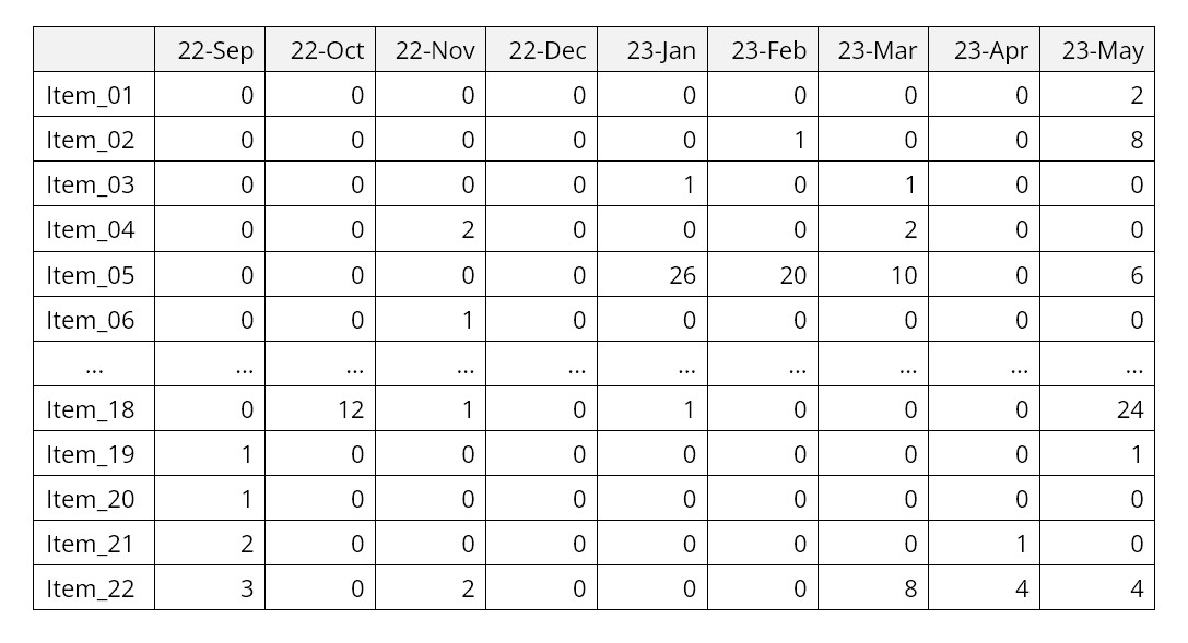
We often post about the benefits of converting parts usage data into smart inventory management decisions. Advanced probability modeling supports generation of realistic demand scenarios that feed into detailed Monte Carlo simulations that expose the consequences of decisions such as choices of Min and Max governing the replenishment of spares.

However, all that new and shiny analytical tech requires quality data as fuel for the analysis. For some public utilities of all kinds, record keeping is not a strong suit, so the raw material going into analysis can be corrupted and misleading. We recently chanced upon documentation of a stark example of this problem at a nuclear power plant (see Scala, ­­­­­­­Needy and Rajgopal: Decision making and tradeoffs in the management of spare parts inventory at utilities. American Association of Engineering Management, 30th ASEM National Conference, Springfield, MO. October 2009). Scala et al. documented the usage history of a critical part whose absence would result in either a facility de-rate or a shutdown. The plant’s usage record for that part spanned more than eight years of data. During that time, the official usage history reported nine events in which positive demand occurred with sizes ranging from one to six units each. There were also five events marked by negative demands (i.e., returns to warehouse) ranging from one to three units each. Careful sleuthing discovered that the true usage occurred in just two events, both with demand of two units. Obviously, calculating the best Min/Max values for this item requires accurate demand data.

The Special Problem of Health and Safety

In the context of “regular” businesses, shortages of spare parts can damage both current revenue and future revenue (related to reputation as a reliable supplier). For an electric utility, however, Scala et al. noted a much greater level of consequence attached to stockouts of spare parts. These include not only a heightened financial and reputational risk but also risks to health and safety: “Ramifications of not having a part in stock include the possibility of having to reduce output or quite possibly, even a plant shut down. From a more long-term perspective, doing so might interrupt the critical service of power to residential, commercial, and/or industrial customers, while damaging the company’s reputation, reliability, and profitability. An electric utility makes and sells only one product: electricity. Losing the ability to sell electricity can be seriously damaging to the company’s bottom line as well its long-term viability.”

All the more reason for electric utilities to be leaders rather than laggards in the deployment of the most advanced probability models for demand forecasting and inventory optimization.

Outside of work, you may have heard the famous dictum “Correlation is not causation.” It may sound like a piece of theoretical fluff that, though involved in a recent Noble Prize in economics, isn’t relevant to your work as a demand planner. Is so, you may be only partially correct.

Extrapolative vs Causal Models

Most demand forecasting uses extrapolative models. Also called time-series models, these forecast demand using only the past values of an item’s demand. Plots of past values reveal trend and seasonality and volatility, so there is a lot they are good for. But there is another type of model – causal models —that can potentially improve forecast accuracy beyond what you can get from extrapolative models.

Causal models bring more input data to the forecasting task: information on presumed forecast “drivers” external to the demand history of an item. Examples of potentially useful causal factors include macroeconomic variables like the inflation rate, the rate of GDP growth, and raw material prices. Examples not tied to the national economy include industry-specific growth rates and your own and competitors’ ad spending.  These variables are usually used as inputs to regression models, which are equations with demand as an output and causal variables as inputs.

Forecasting using Causal Models

Many firms have an S&OP process that involves a monthly review of statistical (extrapolative) forecasts in which management adjusts forecasts based on their judgement. Often this is an indirect and subjective way to work causal models into the process without doing the regression modeling.

To actually make a causal regression model, first you have to nominate a list of potentially-useful causal predictor variables. These may come from your subject matter expertise. For example, suppose you manufacture window glass. Much of your glass may end up in new homes and new office buildings. So, the number of new homes and offices being built are plausible predictor variables in a regression equation.

There is a complication here: if you are using the equation to predict something, you must first predict the predictors. For example, sales of glass next quarter may be strongly related to numbers of new homes and new office buildings next quarter. But how many new homes will there be next quarter? That’s its own forecasting problem. So, you have a potentially powerful forecasting model, but you have extra work to do to make it usable.

There is one way to simplify things: if the predictor variables are “lagged” versions of themselves. For example, the number of new building permits issued six months ago may be a good predictor of glass sales next month. You don’t have to predict the building permit data – you just have to look it up.

Is it a causal relationship or just a spurious correlation?

Causal models are the real deal: there is an actual mechanism that relates the predictor variable to the predicted variable. The example of predicting glass sales from building permits is an example.

A correlation relationship is more iffy. There is a statistical association that may or may not provide a solid basis for forecasting. For example, suppose you sell a product that happens to appeal most strongly to Dutch people but you don’t realize this. The Dutch are, on average, the tallest people in Europe. If your sales are increasing and the average height of Europeans is increasing, you might use that relationship to good effect. However, if the proportion of Dutch in the Euro zone is decreasing while the average height is increasing because the mix of men versus women is shifting toward men, what can go wrong? You will expect sales to increase because average height is increasing. But your sales are really mostly to the Dutch, and their relative share of the population is shrinking, so your sales are really going to decrease instead. In this case the association between sales and customer height is a spurious correlation.

How can you tell the difference between true and spurious relationships? The gold standard is to do a rigorous scientific experiment. But you are not likely to be in position to do that. Instead, you have to rely on your personal “mental model” of how your market works. If your hunches are right, then your potential causal models will correlate with demand and causal modeling will pay off for you, either to supplement extrapolative models or to replace them.

We recently met with the IT team at one of our customers to discuss data requirements and installation of our API based integration that would pull data from their on-premises installation of their ERP system.   The IT manager and analyst both expressed significant concern about providing this data and seriously questioned why it needed to be provided at all.  They even voiced concerns that their data might be resold to their competition. Their reaction was a big surprise to us.  We wrote this blog with them in mind and to make it easier for others to communicate why certain data is necessary to support an effective demand planning process. 

Please note that if you are a forecast analyst, demand planner, of supply chain professional then most of what you’ll read below will be obvious.  But what this meeting taught me is that what is obvious to one group of specialists isn’t going to be obvious to another group of specialists in an entirely different field. 

The Four main types of data that are needed are:  

1. Historical transactions, such as sales orders and shipments.
2. Job usage transactions, such as what components are needed to produce finished goods
3. Inventory Transfer transactions, such as what inventory was shipped from one location to another.
4. Pricing, costs, and attributes, such as the unit cost paid to the supplier, the unit price paid by the customer, and various meta data like product family, class, etc.  

Below is a brief explanation of why this data is needed to support a company’s implementation of demand planning software.

Transactional records of historical sales and shipments by customer
Think of what was drawn out of inventory as the “raw material” required by demand planning software.  This can be what was sold to whom and when or what you shipped to whom and when.  Or what raw materials or subassemblies were consumed in work orders and when.  Or what is supplied to a satellite warehouse from a distribution center and when.

The history of these transactions is analyzed by the software and used to produce statistical forecasts that extrapolate observed patterns.  The data is evaluated to uncover patterns such as trend, seasonality, cyclical patterns, and to identify potential outliers that require business attention.  If this data is not generally accessible or updated in irregular intervals, then it is nearly impossible to create a good prediction of the future demand.  Yes, you could use business knowledge or gut feel but that doesn’t scale and nearly always introduces bias into the forecast (i.e., consistently forecasting too high or too low). 

Data is needed at the transactional level to support finer grained forecasting at the weekly or even daily levels.  For example, as a business enters its busy season it may want to start forecasting weekly to better align production to demand.  You can’t easily do that without having the transactional data in a well-structured data warehouse. 

It might also be the case that certain types of transactions shouldn’t be included in demand data.  This can happen when demand results from a steep discount or some other circumstance that the supply chain team knows will skew the results.  If the data is provided in the aggregate, it is much harder to segregate these exceptions.  At Smart Software, we call the process of figuring out which transactions (and associated transactional attributes) should be counted in the demand signal as “demand signal composition.” Having access to all the transactions enables a company to modify their demand signal as needed over time within the software.  Only providing some of the data results in a far more rigid demand composition that can only be remedied with additional implementation work.

Pricing and Costs
The price you sold your products for and the cost you paid to procure them (or raw materials) is critical to being able to forecast in revenue or costs.  An important part of the demand planning process is getting business knowledge from customers and sales teams.  Sales teams tend to think of demand by customer or product category and speak in the language of dollars.  So, it is important to express a forecast in dollars.  The demand planning system cannot do that if the forecast is shown in units only. 

Often, the demand forecast is used to drive or at least influence a larger planning & budgeting process and the key input to a budget is a forecast of revenue.  When demand forecasts are used to support the S&OP process, the Demand Planning software should either average pricing across all transactions or apply “time-phased” conversions that consider the price sold at that time.   Without the raw data on pricing and costs, the demand planning process can still function, but it will be severely impaired. 

Product attributes, Customer Details, and Locations
Product attributes are needed so that forecasters can aggregate forecasts across different product families, groups, commodity codes, etc. It is helpful to know how many units and total projected dollarized demand for different categories.  Often, business knowledge about what the demand might be in the future is not known at the product level but is known at the product family level, customer level, or regional level.  With the addition of product attributes to your demand planning data feed, you can easily “roll up” forecasts from the item level to a family level.  You can convert forecasts at these levels to dollars and better collaborate on how the forecast should be modified.  

Once the knowledge is applied in the form of a forecast override, the software will automatically reconcile the change to all the individual items that comprise the group.  This way, a forecast analyst doesn’t have to individually adjust every part.  They can make a change at the aggregate level and let the demand planning software do the reconciliation for them. 

Grouping for ease of analysis also applies to customer attributes, such as assigned salesperson or a customer’s preferred ship from location.  And location attributes can be useful, such as assigned region.  Sometimes attributes relate to a product and location combination, like preferred supplier or assigned planner, which can differ for the same product depending on warehouse.

A final note on confidentiality

Recall that our customer expressed concern that we might sell their data to a competitor. We would never do that. For decades, we have been using customer data for training purposes and for improving our products. We are scrupulous about safeguarding customer data and anonymizing anything that might be used, for instance, to illustrate a point in a blog post.

Here are examples of forecasting problems that SmartForecasts can solve, along with the kinds of business data representative of each.

Forecasting an item based on its pattern

Given the following six quarterly sales figures, what sales can you expect for the third and fourth quarters of 2023?

Sales by Quarter

SmartForecasts gives you many ways to approach this problem. You can make your own statistical forecasts using any of six different exponential smoothing and moving average methods. Or, like most nontechnical forecasters, you can use the time-saving Automatic command, which has been programmed to automatically select and use the most accurate method for your data. Finally, to incorporate your business judgment into the forecasting process, you can graphically adjust any statistical forecast result using SmartForecasts’ “eyeball” adjustment capabilities.

Forecasting an item based on its relationship to other variables.

Given the following historical relationship between unit sales and the number of sales representatives, what sales levels can you expect when the planned increase in sales staff takes place over the final two quarters of 2023?

Sales and Sales Representatives by Quarter

You can answer a question like this using SmartForecasts’ powerful Regression command, designed specifically to facilitate forecasting applications that require regression analysis solutions. Regression models with an essentially unlimited number of independent/predictor variables are possible, although most useful regression models use only a handful of predictors.

Simultaneously forecasting a number of product items and their total

Given the following total sales for all dress shirts and the distribution of sales by color, what will individual and total sales be over the next six months?

Monthly Dress Shirt Sales by Color

SmartForecasts’ unique Group Forecasting features automatically and simultaneously forecasts closely related time series, such as these items in the same product group. This saves considerable time and provides forecast results not only for the individual items but also for their total. “Eyeball” adjustments at both the item and group levels are easy to make. You can quickly create forecasts for product groups with hundreds or even thousands of items.

Forecasting thousands of items automatically

Given the following record of product demand at the SKU level, what can you expect demand to be over the next six months for each of the 5,000 SKUs?

Monthly Product Demand by SKU (Stock Keeping Unit)

In just a few minutes, SmartForecasts’ powerful Automatic Selection can take a forecasting job of this size, read the product demand data, automatically create statistical forecasts for each SKU, and saves the result. The results are then ready for export to your ERP system leveraging any one of our API-based connectors or via file export.  Once set up, forecasts will automatically be produced each planning cycle without intervention by the user.

Forecasting demand that is most often zero

A distinct and especially challenging type of data to forecast is intermittent demand, which is most often zero but jumps up to random nonzero values at random times. This pattern is typical of demand for slow moving items, such as service parts or big ticket capital goods.

For example, consider the following sample of demand for aircraft service parts. Note the preponderance of zero values with nonzero values mixed in, often in bursts.

SmartForecasts has a unique method designed especially for this type of data: the Intermittent Demand forecasting feature. Since intermittent demand arises most often in the context of inventory control, this feature focuses on forecasting the range of likely values for the total demand over a lead time, e.g., cumulative demand over the period Jun-23 to Aug-23 in the example above.

Forecasting inventory requirements

Forecasting inventory requirements is a specialized variant of forecasting that focuses on the high end of the range of possible future values.

For simplicity, consider the problem of forecasting inventory requirements for just one period ahead, say one day ahead. Usually, the forecasting job is to estimate the most likely or average level of product demand. However, if available inventory equals the average demand, there is about a 50% chance that demand will exceed inventory, resulting in lost sales and/or lost good will. Setting the inventory level at, say, ten times the average demand will probably eliminate the problem of stockouts, but will just as surely result in bloated inventory costs.

The trick of inventory optimization is to find a satisfactory balance between having enough inventory to meet most demand without tying up too many resources in the process. Usually, the solution is a blend of business judgment and statistics. The judgmental part is to define an acceptable inventory service level, such as meeting 95% of demand immediately from stock. The statistical part is to estimate the 95th percentile of demand.

When not dealing with intermittent demand, SmartForecasts estimates the required inventory level by assuming a bell-shaped (Normal) curve of demand, estimating both the middle and the width of the bell curve, then using a standard statistical formula to estimate the desired percentile. The difference between the desired inventory level and the average level of demand is called the safety stock because it protects against the possibility of stockouts.

When dealing with intermittent demand, the bell-shaped curve is a poor approximation to the statistical distribution of demand. In this special case, SmartForecasts uses patented intermittent demand forecasting technology to estimate the required inventory service level.