Every field, including forecasting, accumulates folk wisdom that eventually starts masquerading as “best practices.”  These best practices are often wise, at least in part, but they often lack context and may not be appropriate for certain customers, industries, or business situations.  There is often a catch, a “Yes, but”. This note is about six usually true forecasting precepts that nevertheless do have their caveats.

1. Organize your company around a one-number forecast. This sounds sensible: it’s good to have a shared vision. But each part of the company will have its own idea about which number is the number. Finance may want quarterly revenue, Marketing may want web site visits, Sales may want churn, Maintenance may want mean time to failure. For that matter, each unit probably has a handful of key metrics. You don’t need a slogan – you need to get your job done.

2. Incorporate business knowledge into a collaborative forecasting process. This is a good general rule, but if your collaborative process is flawed, messing with a statistical forecast via management overrides can decrease accuracy. You don’t need a slogan – you need to measure and compare the accuracy of any and all methods and go with the winners.

3. Forecast using causal modeling. Extrapolative forecasting methods take no account of the underlying forces driving your sales, they just work with the results. Causal modeling takes you deeper into the fundamental drivers and can improve both accuracy and insight. However, causal models (implemented through regression analysis) can be less accurate, especially when they require forecasts of the drivers (“predictions of the predictors”) rather than simply plugging in recorded values of lagged predictor variables. You don’t need a slogan: You need a head-to-head comparison.

4. Forecast demand instead of shipments. Demand is what you really want, but “composing a demand signal” can be tricky: what do you do with internal transfers? One-off’s?  Lost sales? Furthermore, demand data can be manipulated.  For example, if customers intentionally don’t place orders or try to game their orders by ordering too far in advance, then order history won’t be better than shipment history.  At least with shipment history, it’s accurate:  You know what you shipped. Forecasts of shipments are not forecasts of  “demand”, but they are a solid starting point.

5. Use Machine Learning methods. First, “Machine learning” is an elastic concept that includes an ever-growing set of alternatives. Under the hood of many ML advertised models is just an auto-pick an extrapolative forecast method (i.e., best fit) which while great at forecasting normal demand, has been around since the 1980’s (Smart Software was the first company to release an auto-pick method for the PC).   ML models are data hogs that require larger data sets than you may have available. Properly choosing then training an ML model requires a level of statistical expertise that is uncommon in many manufacturing and distribution businesses. You might want to find somebody to hold your hand before you start playing this game.

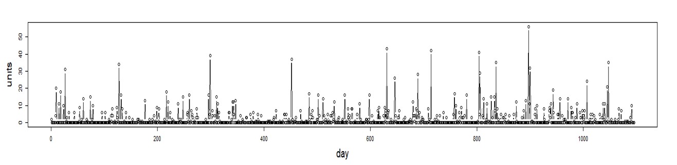
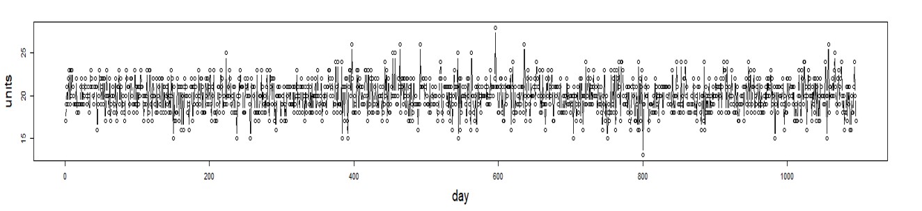
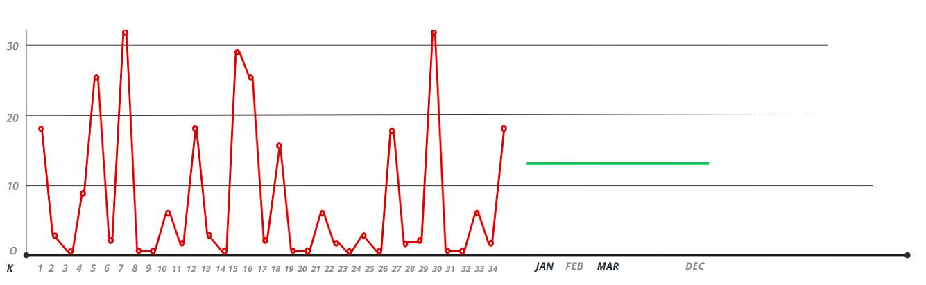
6. Removing outliers creates better forecasts. While it is true that very unusual spikes or drops in demand will mask underlying demand patterns such as trend or seasonality, it isn’t always true that you should remove the spikes. Often these demand surges reflect the uncertainty that can randomly interfere with your business and thus need to be accounted for.  Removing this type of data from your demand forecast model might make the data more predictable on paper but will leave you surprised when it happens again. So, be careful about removing outliers, especially en masse.

Customers often ask us why a stocking recommendation is “so high.” Here is a question we received recently:

During our last team meeting, we found a few items with abnormal gaps between our current ROP and the Smart-suggested ROP at a 99% service level. The concern is that the system indicates that the reorder point will have to increase substantially to achieve a 99% service level. Would you please help us understand the calculation?

When we reviewed the data, it was clear to the customer that the Smart-calculated ROP was indeed correct.  We concluded (1) what they really wanted was a much lower service level target and (2) we had not done a good explaining what was really meant by “service level.” 

So, what does a “99% service level” really mean? 

When it pertains to the target that you enter in your inventory optimization software, it means that the stocking level for the item in question will have a 99% chance of being able to fill whatever the customer needs right away.  For instance, if you have 50 units in stock, there is a 99% chance that the next demand will fall somewhere in the range of 0 to 50 units.

What our customer meant was that 99% of the time a customer placed an order, it was delivered in full within whatever lead time the customer was quoted.  In other words, not necessarily right away but when promised.  

Obviously, the more time you give yourself to deliver to a customer the higher your service level will be. But that distinction is often not explicitly understood when new users of inventory optimization software are conducting what-if scenarios at different service levels.  And that can lead to considerable confusion.  Computing service levels based on immediate stock availability is a higher standard: harder to meet but much more competitive.

Our manufacturing customers often quote service levels based on lead times to their customers, so it isn’t essential for them to deliver immediately from the shelf. In contrast, our customers in the distribution, Maintenance Repair and Operations (MRO), and spare parts spaces, must normally ship same day or within 24 hours.  For them it is a competitive necessity to ship right away and do so in full.

When inputting target service levels using your inventory optimization software, keep this distinction in mind.  Choose the service level based on the percentage of the time you want to ship inventory in full, right away from the shelf.  

Automatic forecasting is the most popular and most used feature of SmartForecasts and Smart Demand Planner. Creating Automatic forecasts is easy. But, the simplicity of Automatic Forecasting masks a powerful interaction of a number of highly effective methods of forecasting. In this blog, we discuss some of the theory behind this core feature. We focus on Automatic forecasting, in part because of its popularity and in part because many other forecasting methods produce similar outputs. Knowledge of Automatic forecasting immediately carries over to Simple Moving Average, Linear Moving Average, Single Exponential Smoothing, Double Exponential Smoothing, Winters’ Exponential Smoothing, and Promo forecasting.

Forecasting tournament

Automatic forecasting works by conducting a tournament among a set of competing methods. Because personal computers and cloud computing are fast, and because we have coded very efficient algorithms into the SmartForecasts’ Automatic forecasting engine, it is practical to take a purely empirical approach to deciding which extrapolative forecasting method to use. This means that you can afford to try out a number of approaches and then retain the one that does best at forecasting the particular data series at hand. SmartForecasts fully automates this process for you by trying the different forecasting methods in a simulated forecasting tournament. The winner of the tournament is the method that comes closest to  predicting new data values from old. Accuracy is measured by average absolute error (that is, the average error, ignoring any minus signs). The average is computed over a set of forecasts, each using a portion of the data, in a process known as sliding simulation.

Sliding simulation

The sliding simulation sweeps repeatedly through ever-longer portions of the historical data, in each case forecasting ahead the desired number of periods in your forecast horizon. Suppose there are 36 historical data values and you need to forecast six periods ahead. Imagine that you want to assess the forecast accuracy of some particular method, say a moving average of four observations, on the data series at hand.

At one point in the sliding simulation, the first 24 points (only) are used to forecast the 25th through 30th historical data values, which we temporarily regard as unknown. We say that points 25-30 are “held out” of the analysis. Computing the absolute values of the differences between the six forecasts and the corresponding actual historical values provides one instance each of a 1-step, 2-step, 3-step, 4-step, 5-step, and 6-step ahead absolute forecast error. Repeating this process using the first 25 points provides more instances of 1-step, 2-step, 3-step ahead errors, and so on. The average over all of the absolute error estimates obtained this way provides a single-number summary of accuracy.

Methods used in Automatic forecasting

Normally, there are six extrapolative forecasting methods competing in the Automatic forecasting tournament:

• Simple moving average
• Linear moving average
• Single exponential smoothing
• Double exponential smoothing
• Additive version of Winters’ exponential smoothing
• Multiplicative version of Winters’ exponential smoothing

The latter two methods are appropriate for seasonal series; however, they are automatically excluded from the tournament if there are fewer than two full seasonal cycles of data (for example, fewer than 24 periods of monthly data or eight periods of quarterly data).

These six classical, smoothing-based methods have proven themselves to be easy to understand, easy to compute and accurate. You can exclude any of these methods from the tournament if you have a preference for some of the competitors and not others.

Lead time delays and supply variability are supply chain facts of life, yet inventory-carrying organizations are often caught by surprise when a supplier is late. An effective inventory planning process embraces this fact of life and develops policies that effectively account for this uncertainty. Sure, there will be times when lead time delays come out of nowhere and cause a shortage. But most often, the shortages result from:

1. Not computing stocking policies (e.g., reorder points, safety stocks, and Min/Max levels) often enough to catch changes in the lead time. 
2. Using poor estimates of actual lead time such as using only averages of historical receipts or relying on a supplier quote.

Instead, recalibrate policies across every single part during every planning cycle to catch changes in demand and lead times.  Rather than assuming only an average lead time, simulate the lead times using scenarios.  This way, recommended stocking policies account for the probabilities of lead times being high and adjust accordingly.  When you do this, you’ll identify needed inventory increases before it is too late. You’ll capture more sales and drive significant improvements in customer satisfaction.

Managing spare parts presents numerous challenges, such as unexpected breakdowns, changing schedules, and inconsistent demand patterns. Traditional forecasting methods and manual approaches are ineffective in dealing with these complexities. To overcome these challenges, this blog outlines key strategies that prioritize service levels, utilize probabilistic methods to calculate reorder points, regularly adjust stocking policies, and implement a dedicated planning process to avoid excessive inventory. Explore these strategies to optimize spare parts inventory and improve operational efficiency.

Bottom Line Upfront

​1.Inventory Management is Risk Management.

2.Can’t manage risk well or at scale with subjective planning – Need to know service vs. cost.

3.It’s not supply & demand variability that are the problem – it’s how you handle it.

4.Spare parts have intermittent demand so traditional methods don’t work.

5.Rule of thumb approaches don’t account for demand variability and misallocate stock.

6.Use Service Level Driven Planning  (service vs. cost tradeoffs) to drive stock decisions.

7.Probabilistic approaches such as bootstrapping yield accurate estimates of reorder points.

8.Classify parts and assign service level targets by class.

9.Recalibrate often – thousands of parts have old, stale reorder points.

10.Repairable parts require special treatment.

Do Focus on the Real Root Causes

Intermittent Demand

• Slow moving, irregular or sporadic with a large percentage of zero values.
• Non-zero values are mixed in randomly – spikes are large and varied.
• Isn’t bell shaped (demand is not Normally distributed around the average.)
• At least 70% of a typical Utility’s parts are intermittently demanded.

Normal Demand

• Very few periods of zero demand (exception is seasonal parts.)
• Often exhibits trend, seasonal, or cyclical patterns.
• Lower levels of demand variability.
• Is bell-shaped (demand is Normally distributed around the average.)

Don’t rely on averages

• OK for determining typical usage over longer periods of time.
• Often forecasts more “accurately” than some advanced methods.
• But…insufficient for determining what to stock.

Don’t Buffer with Multiples of Averages

Example:  Two equally important parts so let’s treat them the same.
We’ll order more  when On Hand Inventory ≤ 2 x Avg Lead Time Demand.

Do use Service Level tradeoff curves to compute safety stock

Standard Normal Probabilities

OK for normal demand. Doesn’t work with intermittent demand!

Don’t use Normal (Bell Shaped) Distributions

• You’ll get the tradeoff curve wrong:

– e.g., You’ll target 95% but achieve 85%.

– e.g., You’ll target 99% but achieve 91%.

• This is a huge miss with costly implications:

– You’ll stock out more often than expected.

– You’ll start to add subjective buffers to compensate and then overstock.

– Lack of trust/second-guessing of outputs paralyzes planning.

Why Traditional Methods Fail on Intermittent Demand: 

Traditional Methods are not designed to address core issues in spare parts management.

Need: Probability distribution (not bell-shaped) of demand over variable lead time.

• Get: Prediction of average demand in each month, not a total over lead time.
• Get: Bolted-on model of variability, usually the Normal model, usually wrong.

Need: Exposure of tradeoffs between item availability and cost of inventory.

• Get: None of this; instead, get a lot of inconsistent, ad-hoc decisions.

Do use Statistical Bootstrapping to Predict the Distribution:

Then exploit the distribution to optimize stocking policies.

How does Bootstrapping Work?

24 Months of Historical Demand Data.

Bootstrap Scenarios for a 3-month Lead Time.

Bootstrapping Hits the Service Level Target with nearly 100% Accuracy!

• National Warehousing Operation.

Task: Forecast inventory stocking levels for 12,000 intermittently demanded SKUs at 95% & 99% service levels

Results:

At 95% service level, 95.23% did not stock out.

At 99% service level, 98.66% did not stock out.

This means you can rely on output to set expectations and confidently make targeted stock adjustments that lower inventory and increase service.

Set Target Service Levels According to Order Frequency & Size

Recalibrate Reorder Points Frequently

• Static ROPs cause excess and shortages.
• As lead time increases, so should the ROP and vice versa.
• As usage decreases, so should the ROP and vice versa.
• Longer you wait to recalibrate, the greater the imbalance.
• Mountains of parts ordered too soon or too late.
• Wastes buyers’ time placing the wrong orders.
• Breeds distrust in systems and forces data silos.

Do Plan Rotables (Repair Parts) Differently

Summary

1.Inventory Management is Risk Management.

2.Can’t manage risk well or at scale with subjective planning – Need to know service vs. cost.

3.It’s not supply & demand variability that are the problem – it’s how you handle it.

4.Spare parts have intermittent demand so traditional methods don’t work.

5.Rule of thumb approaches don’t account demand variability and misallocate stock.

6.Use Service Level Driven Planning  (service vs. cost tradeoffs) to drive stock decisions.

7.Probabilistic approaches such as bootstrapping yield accurate estimates of reorder points.

8.Classify parts and assign service level targets by class.

9.Recalibrate often – thousands of parts have old, stale reorder points.

10.Repairable parts require special treatment.