Forecast accuracy is a key metric by which to judge the quality of your demand planning process. (It’s not the only one. Others include timeliness and cost; See 5 Demand Planning Tips for Calculating Forecast Uncertainty.) Once you have forecasts, there are a number of ways to summarize their accuracy, usually designated by obscure three- or four-letter acronyms like MAPE, RMSE, and MAE.  See Four Useful Ways to Measure Forecast Error for more detail.

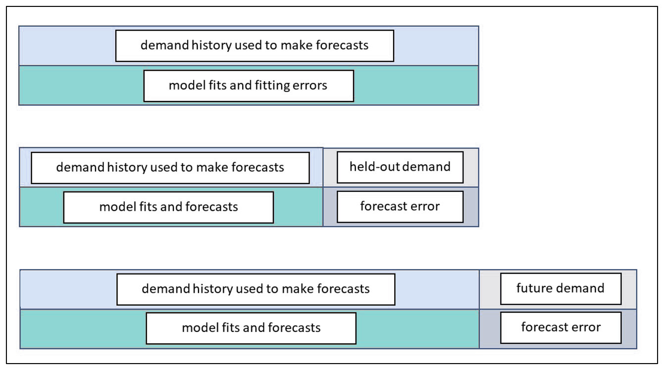
A less discussed but more fundamental issue is how computational experiments are organized for computing forecast error. This post compares the three most important experimental designs. One of them is old-school and essentially amounts to cheating. Another is the gold standard. A third is a useful expedient that mimics the gold standard and is best thought of as predicting how the gold standard will turn out. Figure 1 is a schematic view of the three methods.

Figure 1: Three ways to assess forecast error

The top panel of Figure 1 depicts the way forecast error was assessed back in the early 1980’s before we moved the state of the art to the scheme shown in the middle panel. In the old days, forecasts were assessed on the same data used to compute the forecasts. After a model was fit to the data, the errors computed were not for model forecasts but for model fits. The difference is that forecasts are for future values, while fits are for concurrent values. For example, suppose the forecasting model is a simple moving average of the three most recent observations. At time 3, the model computes the average of observations 1, 2, and 3. This average would then be compared to the observed value at time 3. We call this cheating because the observed value at time 3 got a vote on what the forecast should be at time 3. A true forecast assessment would compare the average of the first three observations to the value of the next, fourth, observation. Otherwise, the forecaster is left with an overly optimistic assessment of forecast accuracy.

The bottom panel of Figure 1 shows the best way to assess forecast accuracy. In this schema, all the historical demand data are used to fit a model, which is then used to forecast future, unknown demand values. Eventually, the future unfolds, the true future values reveal themselves, and actual forecast errors can be computed. This is the gold standard. This information populates the “forecasts versus actuals” report in our software.

The middle panel depicts a useful halfway measure. The problem with the gold standard is that you must wait to learn how well your chosen forecasting methods perform. This delay does not help when you are required to choose, in the moment, which forecasting method to use for each item. Nor does it provide a timely estimate of the forecast uncertainty you will experience, which is important for risk management such as forecast hedging. The middle way is based on hold-out analysis, which excludes (“holds out”) the most recent observations and asks the forecasting method to do its work without knowing those ground truths. Then the forecasts based on the foreshortened demand history can be compared to the held-out actual values to get an honest assessment of forecast error.

“Despite what you’ve seen in your Saturday morning cartoons, elephants can’t jump, and there’s one simple reason: They don’t have to. Most jumpy animals—your kangaroos, monkeys, and frogs—do it primarily to get away from predators.”  — Patrick Monahan, Science.org, Jan 27, 2016.

Now you know why the largest ERP companies can’t develop high quality best-of-breed like solutions. They never had to, so they never evolved to innovate outside of their core focus. 

However, as ERP systems have become commoditized, gaps in their functionality became impossible to ignore. The larger players sought to protect their share of customer wallet by promising to develop innovative add-on applications to fill all the white spaces.  But without that “innovation muscle,” many projects failed, and mountains of technical debt accumulated.

Best-of-breed companies evolved to innovate and have deep functional expertise in specific verticals.  The result is that best of breed ERP add-ons are easier to use, have more features, and deliver more value than the native ERP modules they replace. 

If your ERP provider has already partnered with an innovative best of breed add-on provider*, you’re all set! But if you can only get the basics from your ERP, go with a best-of-breed add-on that has a bespoke integration to the ERP. 

A great place to start your search is to look for ERP demand planning add-ons that add brains to the ERP’s brawn, i.e., those that support inventory optimization and demand forecasting.  Leverage add-on tools like Smart’s statistical forecasting, demand planning, and inventory optimization apps to develop forecasts and stocking policies that are fed back to the ERP system to drive daily ordering. 

*App-stores are a license for the best of breed to sell into the ERP companies base –  being listed  partnerships.

There’s one thing I’m reminded of almost every day at Smart Software that puzzle me: most companies do not understand how forecasts are created, and stocking policies are determined.  It’s an organizational black box. Here is an example from a recent sales call:

How do you forecast?
We use history.

How do you use history?
What do you mean?

Well, you can take an average of the last year, last two years, average the most recent periods, or use some other type of formula to generate the forecast.
I’m pretty sure we use an average of the last 12 months.

Why 12 months instead of a different amount of history?
12 months is a good amount of time to use because it doesn’t get skewed by older data but it’s recent enough

How do you know it’s more accurate than using 18 months or some other length of history?
We don’t know. We do adjust the forecasts based on feedback from sales.  

Do you know if the adjustments make things more accurate or less than if you just used the average?
We don’t know but are confident that forecasts are inflated

What do the inventory buyers do then if they think the numbers are inflated?
They have lots of business knowledge and adjust their buys accordingly

So, is it fair to say they would ignore the forecasts at least some of the time?
Yes, some of the time.

How do the buyers decide when to order more? Do you have a reorder point or safety stock specified in your ERP system that helps guide these decisions?
Yes, we use a safety stock field.

How is safety stock calculated?
Buyers determine this based on the importance of the item, lead times, and other considerations such as how many customers purchase the item, the velocity of the item, it’s cost.  They’ll carry different amounts of safety stock depending on this.

The discussion continued. The main takeaway here is that when you scratch just below the surface, far more questions are revealed than answers.  This often means that the inventory planning and demand forecast process is highly subjective, varies from planner to planner, is not well understood by the rest of the organization, and likely to be reactive.  As Tom Willemain has described it’s “chaos masked by improvisation.”   The “as-is” process needs to be fully identified and documented.  Only then can gaps be exposed, and improvements can be made.   Here is a list of 10 questions  you can ask that will reveal your organization’s true forecasting, demand planning, and inventory planning process.

In a recent LinkedIn post, I detailed four questions that, when answered, will reveal how forecasts are being used in your business.  In this article, we’ve listed questions you can ask that will reveal how forecasts are created.

1. When we ask users how they create forecasts, their answer will often be “we use history.” This obviously isn’t enough information, as there are different types of demand history that require different forecasting methods. If you are using historical data, then make sure to find out if you are using an averaging model, a trending model, a seasonal model, or something else to forecast.

2. Once you know the model used, ask about the parameter values of those models. The forecast output of an “average” will differ, sometimes significantly, depending on the number of periods you are averaging.  So, find out whether you are using an average of the last 3 months, 6 months, 12 months, etc.

3. If you are using trending models, ask how the model weights are set. For example, in a trending model, such as double exponential smoothing, the forecasts will differ significantly depending on how the calculations weight recent data compared to older data (higher weights put more emphasis on the recent data).

4. If you are using seasonal models, the forecast results are going to be impacted by the “level” and “trending weights” used. You should also determine whether seasonal periods are forecasted with multiplicative or additive seasonality.  (Additive seasonality says, e.g., “Add 100 units for July”, whereas multiplicative seasonality says “Multiply by 1.25 for July.”) Finally, you may not be using these types of methods at all.  Some practitioners will use a forecast method that simply averages prior periods (i.e., next June will be forecasted based on the average of the prior three Junes).

5. How do you go about choosing one model over another? Does the choice of technique depend on the type of demand data or when new demand data are available? Is this process automated? Or if a planner chooses a trend model subjectively, will that item continue to be forecasted with that model until the planner changes it again?

6. Are your forecasts “fully automatic,” so that trend and/or seasonality are detected automatically? Or are your forecasts dependent on item classifications that must be maintained by users? The latter requires more time and attention from planners to define what behavior constitutes trend, seasonality, etc.

7. What are the item classification rules used? For example, an item may be considered a trending item if demand increases by more than 5% period-over-period. An item may be considered seasonal if 70% or more of the annual demand occurs in four or fewer periods. Such rules are user-defined and often require overly broad assumptions. Sometimes they are configured when a system was originally implemented but never revised even as conditions change. It’s important to make sure any classification rules are understood and, if necessary, updated.

8. Does the forecast regenerate automatically when new data are available, or do you have to manually regenerate the forecasts?

9. Do you check for any change in forecast from one period to the next before deciding whether to use the new forecast? Or do you default to the new forecast?

10. How are forecast overrides that were made in prior planning cycles treated when a new forecast is created? Are they reused or replaced?

11. How do you incorporate forecasts made by your sales team or by your customers? Do these forecasts replace the baseline forecast, or do you use these inputs to make planner overrides to the baseline forecast?

12. Under what circumstances would you ignore the baseline forecast and use exactly what sales or customers are telling you?

13. If you rely on customer forecasts, what do you do about customers who don’t provide forecasts?

14. How do you document the effectiveness of your forecasting approach?  Most companies only measure the accuracy of the final forecast that is submitted to the ERP system, if they measure anything. But they don’t assess alternative predictions that might have been used. It is important to compare what you are doing to benchmarks. For example, do the methods you are using outperform a naïve forecast (i.e., “tomorrow equals today,” which requires no thought), or what you saw last year, or the average of the last 12 months.  Benchmarking your baseline forecast insures you are squeezing as much accuracy as possible out of the data.

15. Do you measure whether overrides from sales, customers, and planners are making the forecast better or worse? This is just as important as measuring whether your statistical approaches are outperforming the naïve method.  If you don’t know whether overrides are helping or hurting, the business can’t get better at forecasting – you need to know which steps are adding value so that you can do more of those and get even better. If you aren’t documenting forecast accuracy and conducting “forecast value add” analysis, then you aren’t able to properly assess whether the forecasts being produced are the best you could make.  You’ll miss opportunities to improve the process, increase accuracy, and educate the business on what type of forecast error is to be expected.

Smart IP&O is powered by the SmartForecasts® forecasting engine that automatically selects the most appropriate method for each item.  Smart Forecast methods are listed below:

• Simple Moving Average and Single Exponential Smoothing for flat, noisy data
• Linear Moving Average and Double Exponential Smoothing for trending data
• Winters Additive and Winters Multiplicative for seasonal and seasonal & trending data.

This blog explains how each model works using time plots of historical and forecast data.  It outlines how to go about choosing which model to use.   The examples below show the same history, in red, forecasted with each method, in dark green, compared to the Smart-chosen winning method, in light green.

Seasonality
If you want to force (or prevent) seasonality to show in the forecast, then choose Winters models.  Both methods require 2 full years of history.

`Winter’s multiplicative will determine the size of the peaks or valleys of seasonal effects based on a percentage difference from a trending average volume.  It is not a good fit for very low volume items due to division by zero when determining that percentage. Note in the image below that the large percentage drop in seasonal demand in the history is being projected to continue over the forecast horizon making it look like there isn’t any seasonal demand despite using a seasonal method.

Statistical forecast produced with Winter’s multiplicative method. 

Winter’s additive will determine the size of the peaks or valleys of seasonal effects based on a unit difference from the average volume.  It is not a good fit if there’s significant trend to the data.  Note in the image below that seasonality is now being forecasted based on the average unit change in seasonality. So, the forecast still clearly reflects the seasonal pattern despite the down trend in both the level and seasonal peaks/valleys.

Statistical forecast produced with Winter’s additive method.

Trend

If you want to force (or prevent) trend up or down to show in the forecast, then restrict the chosen methods to (or remove the methods of) Linear Moving Average and Double Exponential Smoothing.

 Double exponential smoothing will pick up on a long-term trend.  It is not a good fit if there are few historical data points.

Statistical forecast produced with Double Exponential Smoothing

Linear moving average will pick up on nearer term trends.  It is not a good fit for highly volatile data

Non-Trending and Non-Seasonal Data
If you want to force (or prevent) an average from showing in the forecast, then restrict the chosen methods to (or remove the methods of) Simple Moving Average and Single Exponential Smoothing.

Single exponential smoothing will weigh the most recent data more heavily and produce a flat-line forecast.  It is not a good fit for trending or seasonal data.

Statistical forecast using Single Exponential Smoothing

Simple moving average will find an average for each period, sometimes appearing to wiggle, and better for longer-term averaging.  It is not a good fit for trending or seasonal data.

Statistical forecast using Simple Moving Average