Managing Inventory amid Regime Change

​If you hear the phrase “regime change” on the news, you immediately think of some fraught geopolitical event. Statisticians use the phrase differently, in a way that has high relevance for demand planning and inventory optimization. This blog is about “regime change” in the statistical sense, meaning a major change in the character of the demand for an inventory item.

An item’s demand history is the fuel that powers demand planners’ forecasting machines. In general, the more fuel the better, giving us a better fix on the average level, the volatility, the size and frequency of any spikes, the shape of any seasonality pattern, and the size and direction of any trend.

But there is one big exception to the rule that “more data is better data.” If there is a major shift in your world and new demand doesn’t look like old demand, then old data become dangerous.

Modern software can make accurate forecasts of item demand and suggest wise choices for inventory parameters like reorder points and order quantities. But the validity of these calculations depends on the relevance of the data used in their calculation. Old data from an old regime no longer reflect current reality, so including them in calculations creates forecast error for demand planners and either excess stock or unacceptable stockout rates for inventory planners.

That said, if you were to endure a recent regime change and throw out the obsolete data, you would have a lot less data to work with. This has its own costs, because all the estimates computed from the data would have greater statistical uncertainty even though they would be less biased. In this case, your calculations would have to rely more heavily on a blend of statistical analysis and your own expert judgement.

At this point, you may ask “How can I know if and when there has been a regime change?” If you’ve been on the job for a while and are comfortable looking at timeplots of item demand, you will generally recognize regime change when you see it, at least if it’s not too subtle. Figure 1 shows some real-world examples that are obvious.

Figure 1 Four examples of regime change in real-world item demand

Figure 1: Four examples of regime change in real-world item demand


Unfortunately, less obvious changes can still have significant effects. Moreover, most of our customers are too busy to manually review all the items they manage even once per quarter. When you get beyond, say, 100 items, the task of eyeballing all those time series becomes onerous. Fortunately, software can do a good job of continuously monitoring demand for tens of thousands of items and alerting you to any items that may need your attention. Then too, you can arrange for the software to not only detect regime change but also automatically exclude from its calculations all data collected before the most recent regime change, if any. In other words, you can get both automatic warning of regime change and automatic protection from regime change.

For more on the basics of regime change, see our previous blog on the topic: https://smartcorp.com/blog/demandplanningregimechange/  


An Example with Numbers in It

If you would like to learn more, read on to see a numerical example of how much regime change can alter the calculation of a reorder point for a critical spare part. Here is a scenario to illustrate the point.

Scenario

  • Goal: calculate the reorder point needed to control the risk of stockout while waiting for replenishment. Assume the target stockout risk is 5%.
  • Assume the item has intermittent daily demand, with many days of zero demand.
  • Assume daily demand has a Poisson distribution with an average of 1.0 units per day.
  • Assume the replenishment lead time is always 30 days.
  • The lead time demand will be random, so it will have a probability distribution and the reorder point will be the 95th percentile of the distribution.
  • Assume the effect of regime change is to either raise or lower the mean daily demand.
  • Assume there is one year of daily data available for estimating the mean daily unit demand.


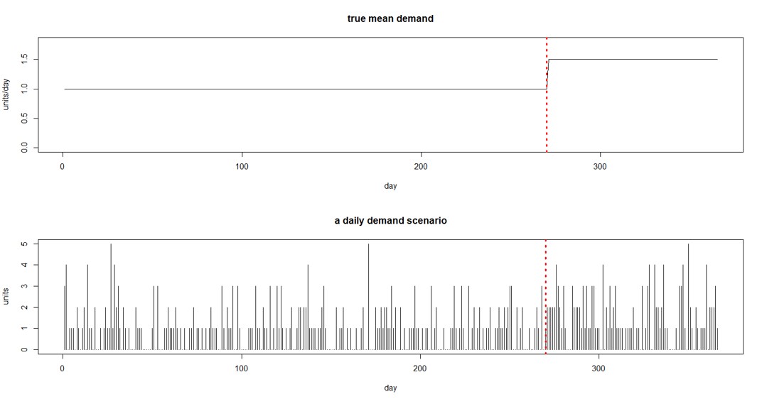
Figure 2 Example of change in mean demand and sample of random daily demand

Figure 2 Example of change in mean demand and sample of random daily demand


Figure 2 shows one form of this scenario. The top panel shows that the average daily demand increases from 1.0 to 1.5 after 270 days. The bottom panel shows one way that a year’s worth of daily demand might appear. (At this point, you may be feeling that calculating all this stuff is complicated, even for what turns out to be a simplified scenario. That is why we have software!)

Analysis

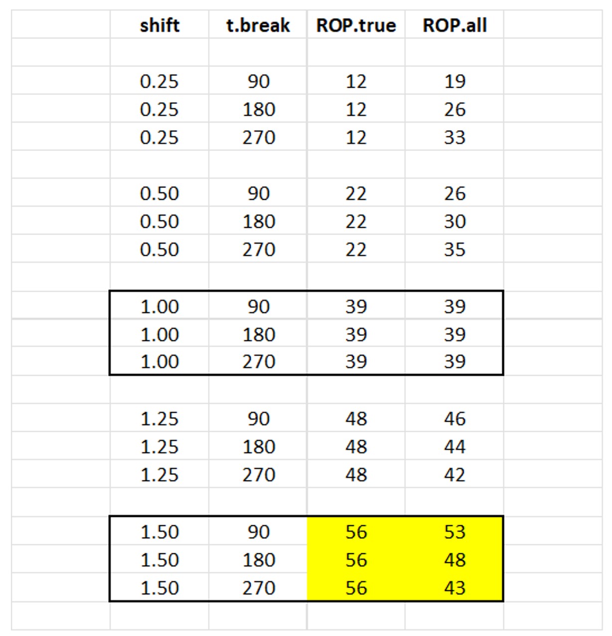
Successful calculation of the proper reorder point will depend on when regime change happens and how big a change occurs. We simulated regime changes of various sizes at various times within a 365 day period. Around a base demand of 1.0 units per day, we studied shifts in demand (“shift”) of ±25% and ±50% as well as a no change reference case. We located the time of the change (“t.break”) at 90, 180, and 270 days. In each case, we computed two estimates of the reorder point: The “ideal” value given perfect knowledge of the average demand in the new regime (“ROP.true”), and the estimated value of mean demand computed by ignoring the regime change and using all the demand data for the past year (“ROP.all”).

Table 1 shows the estimates of the reorder point computed over 100 simulations. The center block is the reference case, in which there is no change in the daily demand, which remains fixed at 1 unit per day. The colored block at the bottom is the most extreme increasing scenario, with demand increasing to 1.5 units/day either one-third, one-half, or two-thirds of the way through the year.

We can draw several conclusions from these simulations.

ROP.true: The correct choice for reorder point increases or decreases according to the change in mean demand after the regime change. The relationship is not a simple linear one: the table spans a 600% range of demand levels (0.25 to 1.50) but a 467% range of reorder points (from 12 to 56).

ROP.all: Ignoring the regime change can lead to gross overestimates of the reorder point when demand drops and gross underestimates when demand increases.  As we would expect, the later the regime change, the worse the error. For example, if demand increases from 1.0 to 1.5 units per day two-thirds of the way through the year without being noticed, the calculated reorder point of 43 units would fall 13 units short of where it should be.

A word of caution: Table 1 shows that basing the calculations of reorder points using only data from after a regime change will usually get the right answer. What it doesn’t show is that the estimates can be unstable if there is very little demand history after the change. Therefore, in practice, you should wait to react to the regime change until a decent number of observations have accumulated in the new regime. This might mean using all the demand history, both pre- and post-change, until, say, 60 or 90 days of history have accumulated before ignoring pre-change data.

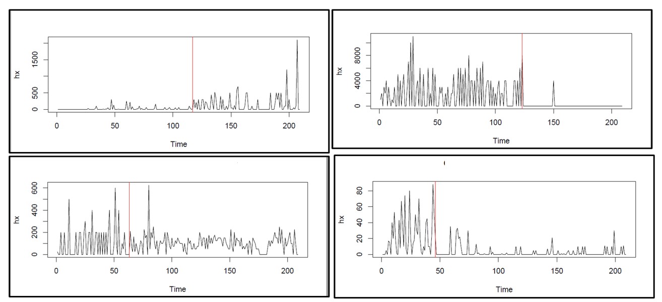
 

Table 1 Correct and Estimated Reorder Points for different regime change scenarios

Table 1 Correct and Estimated Reorder Points for different regime change scenarios

Demand Planning with Blanket Orders

Customer as Teacher

Our customers are great teachers who have always helped us bridge the gap between textbook theory and practical application of forecasting and demand planning. Our latest bit of schooling concerns “blanket orders” and how to account for them as part of the demand planning process. 

Expanding the Inventory Theory Textbook

Textbook inventory theory focuses on the three most used replenishment policies: (1) Periodic review order-up-to policy, designated (T, S) in the books (2) Continuous review policy with fixed order quantity, designated (R, Q) and (3) Continuous review order-up-to policy, designated (s, S) but usually called “Min/Max.” Our customers have pointed out that their actual ordering process often includes frequent use of “blanket orders.” This blog focuses on how to incorporate blanket orders into the demand planning process and details how to adjust stocking targets accordingly.

Demand Planning with Blanket Orders is Different

Blanket orders are contracts with suppliers for fixed replenishment quantities arriving at fixed intervals. For example, you might agree with your supplier to receive 20 units every 7 days via a blanket order rather than 60 to 90 units every 28 days under the Periodic Review policy. Blanket orders contrast even more with the Continuous Review policies, under which both order schedules and order quantities are random.  In general, it is efficient to build flexibility into the restocking process so that you order only what you need and only order when you need it. By that standard, Min/Max should make the most sense and blanket policies should make the least sense.

The Case for Blanket Policies

However, while efficiency is important, it is never the only consideration. One of our customers, let’s call them Company X, explained the appeal of blanket policies in their circumstances. Company X makes high-performance parts for motorcycles and ATV’s. They turn raw steel into cool things.  But they must deal with the steel. Steel is expensive. Steel is bulky and heavy. Steel is not something conjured overnight on a special-order basis. The inventory manager at Company X does not want to place large but random-sized orders at random times. He does not want to baby-sit a mountain of steel. His suppliers do not want to receive orders for random quantities at random times. And Company X prefers to spread out its payments. The result: Blanket orders.

The Fatal Flaw in Blanket Policies

For Company X, blanket orders are intended to even out replenishment buys and avoid unwieldy buildups of piles of steel before they are ready for use. But the logic behind continuous review inventory policies still applies. Surges in demand, otherwise welcome, will occur and can create stockouts. Likewise, pauses in demand can create excess demand. As time goes on, it becomes clear that a blanket policy has a fatal flaw: only if the blanket orders exactly match the average demand can they avoid runaway inventory in either direction, up or down. In practice, it will be impossible to exactly match average demand. Furthermore, average demand is a moving target and can drift up or down.

How to Incorporate Blanket Orders when Demand Planning 

A blanket policy does have advantages, but rigidity is its Achilles heel.  Demand planners will often improvise by adjusting future orders to handle changes in demand but this doesn’t scale across thousands of items.  To make the inventory replenishment policy robust against randomness in demand, we suggest a hybrid policy that begins with blanket orders but retains flexibility to automatically (not manually) order additional supply on an as-need basis. Supplementing the blanket policy with a Min/Max backup provides for adjustments without manual intervention. This combination will capture some of the advantages of blanket orders while protecting customer service and avoiding runaway inventory.

Designing a demand planning process that accounts for blanket orders properly requires choice of four control parameters. Two parameters are the fixed size and fixed timing of the blanket policy. Two more are the values of Min and Max. This leaves the inventory manager facing a four-dimensional optimization problem.  Advanced inventory optimization software will make it possible to evaluate choices for the values of the four parameters and to support negotiations with suppliers when crafting blanket orders.


Optimizing Inventory around Suppliers´ Minimum Order Quantities

Recently, I had an interesting conversation with an inventory manager and the VP Finance. We were discussing the benefits of being able to automatically optimize both reorder points and order quantities. The VP Finance was concerned that given their large supplier required minimum order quantities, they would not be able to benefit.  He said his suppliers held all the power, forcing him to accept massive minimum order quantities and tying his hands. While he felt bad about this, he saw a silver lining: He didn’t have to do any planning. He would accept a large inventory investment, but his customer service levels would be exceptional.  Perhaps the large inventory investment was assumed to be the cost of doing business.

I pushed back and pointed out that he was not as powerless as he felt. He still had control of the other half of the procurement process: while he couldn’t control how much to order, he could control when to order by adjusting the reorder point. In other words, there is always room for careful quantitative analysis in inventory management, even when you have one hand tied behind your back.

An Example

To put some numbers behind my argument, I created a scenario then analyzed it using our methodology to show how consequential it can be to use inventory optimization software even in constrained situations. In this scenario, item demand averages 2.2 units per day but varies significantly by day of week. Let’s say the imaginary supplier insists on a minimum order quantity of 500 units (way out of proportion to demand) and fills replenishment orders in either three days or ten days in equal proportions (quite inconsistent). To spread the blame around, let’s also suppose that the imaginary supplier’s imaginary customer uses a foolish rule that the reorder point should be 10% of the minimum order quantity. (Why this rule? Too many companies use simple/simplistic rules of thumb in lieu of proper analysis.)

So, we have a base case in which the order quantity is 500 units, and the reorder point is 50 units. In this case, the fill rate is 100%, but the average number of units on hand is a whopping 330. If the customer would simply lower the reorder point from 50 to 15, the fill rate would still be 99.5%, but the average stock on hand would drop by 11% to 295 units. Using the one hand not tied behind his back, the inventory manager could cut his inventory investment by more than 10%, which would be a noticeable win.

Incidentally, if the minimum order quantity were abolished, the customer would be free to arrive at a new and much better solution. Setting the order quantity to 45 and the reorder point to 25 would achieve a 99% fill rate at the cost of a daily on-hand level of only 35 units: nearly a 90% reduction in inventory investment: a major improvement over the status quo.

Postscript

These calculations are possible using our software, which can make visible the otherwise unknown relationships between inventory system design choices (e.g., order quantity and reorder point) and key performance indicators (e.g., average units on hand and fill rate).  Armed with this ability to conduct these calculations, alternative arrangements with the supplier may now be considered. For example, what if, in exchange for paying a higher price per unit, the supplier agreed to a lower MOQ. Using the software to conduct an analysis of the key performance indicators using the “what if” costs and MOQs would reveal the cost per unit and MOQ that would be needed to develop a more profitable deal.   Once identified, all parties stand to benefit.  The supplier now generates a better margin on sales of its products, and the buyer holds considerably less inventory yielding a holding cost reduction that dwarfs the added cost per unit.  Everyone wins.


A Beginner’s Guide to Downtime and What to Do about It

This blog provides an overview of this topic written for non-experts. It

  • explains why you might want to read this blog.
  • lists the various types of “machine maintenance.”
  • explains what “probabilistic modeling” is.
  • describes models for predicting downtime.
  • explains what these models can do for you.

Importance of Downtime

If you manufacture things for sale, you need machines to make those things. If your machines are up and running, you have a fighting chance to make money. If your machines are down, you lose opportunities to make money. Since downtime is so fundamental, it is worth some investment of money and thought to minimize downtime. By thought I mean probability math, since machine downtime is inherently a random phenomenon. Probability models can guide maintenance policies.

Machine Maintenance Policies

Maintenance is your defense against downtime. There are multiple types of maintenance policies, ranging from “Do nothing and wait for failure” to sophisticated analytic approaches involving sensors and probability models of failure.

A useful list of maintenance policies is:

  • Sitting back and wait for trouble, then sitting around some more wondering what to do when trouble inevitably happens. This is as foolish as it sounds.
  • Same as above except you prepare for the failure to minimize downtime, e.g., stockpiling spare parts.
  • Periodically checking for impending trouble coupled with interventions such as lubricating moving parts or replacing worn parts.
  • Basing the timing of maintenance on data about machine condition rather than relying on a fixed schedule; requires ongoing data collection and analysis. This is called condition-based maintenance.
  • Using data on machine condition more aggressively by converting it into predictions of failure time and suggestions for steps to take to delay failure. This is called predictive maintenance.

The last three types of maintenance rely on probability math to establish a maintenance schedule, or determine when data on machine condition call for intervention, or calculate when failure might occur and how best to postpone it.


Probability Models of Machine Failure

How long a machine will run before it fails is a random variable. So is the time it will spend down. Probability theory is the part of math that deals with random variables. Random variables are described by their probability distributions, e.g., what is the chance that the machine will run for 100 hours before it goes down? 200 hours? Or, equivalently, what is the chance that the machine is still working after 100 hours or 200 hours?

A sub-field called “reliability theory” answers this type of question and addresses related concepts like Mean Time Before Failure (MTBF), which is a shorthand summary of the information encoded in the probability distribution of time before failure.

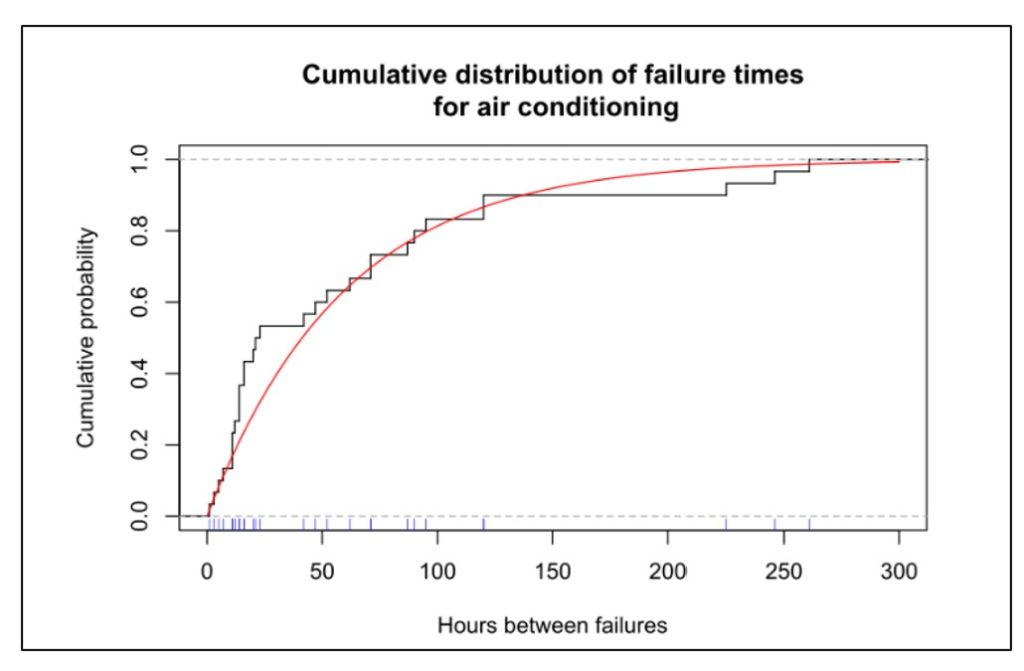
Figures 1 shows data on the time before failure of air conditioning units. This type of plot depicts the cumulative probability distribution and shows the chance that a unit will have failed after some amount of time has elapsed. Figure 2 shows a reliability function, plotting the same type of information in an inverse format, i.e., depicting the chance that a unit is still functioning after some amount of time has elapsed.

In Figure 1, the blue tick marks next to the x-axis show the times at which individual air conditioners were observed to fail; this is the basic data. The black curve shows the cumulative proportion of units failed over time. The red curve is a mathematical approximation to the black curve – in this case an exponential distribution. The plots show that about 80 percent of the units will fail before 100 hours of operation.

Figure 1 Cumulative distribution function of uptime for air conditioners

Figure 1 Cumulative distribution function of uptime for air conditioners


Probability models can be applied to an individual part or component or subsystem, to a collection of related parts (e.g., “the hydraulic system”), or to an entire machine. Any of these can be described by the probability distribution of the time before they fail.

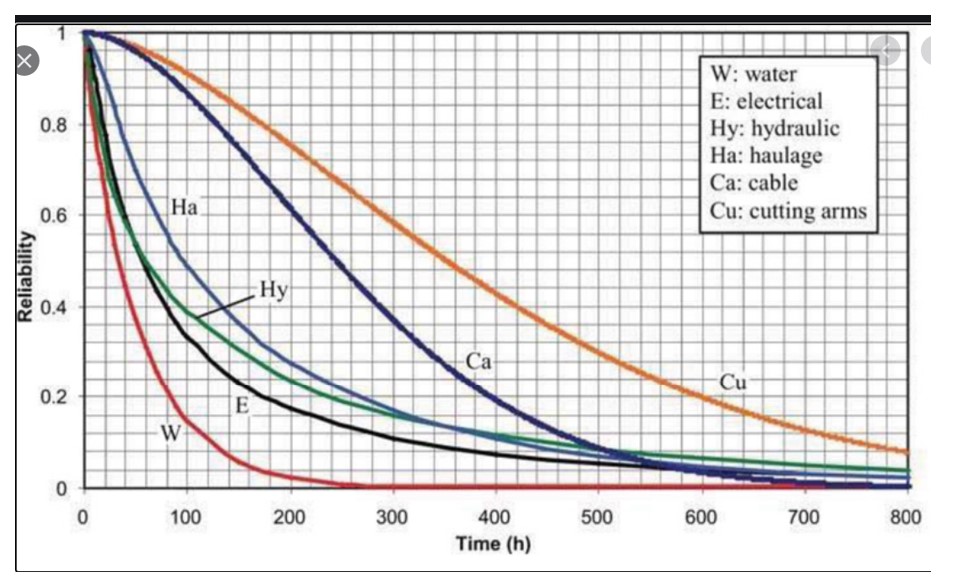
Figure 2 shows the reliability function of six subsystems in a machine for digging tunnels. The plot shows that the most reliable subsystem is the cutting arms and the least reliable is the water subsystem. The reliability of the entire system could be approximated by multiplying all six curves (because for the system as a whole to work, every subsystem must be functioning), which would result in a very short interval before something goes wrong.

Figure 2 Examples of probability distributions of subsystems in a tunneling machine

Figure 2 Examples of probability distributions of subsystems in a tunneling machine


Various factors influence the distribution of the time before failure. Investing in better parts will prolong system life. So will investing in redundancy. So will replacing used pars with new.

Once a probability distribution is available, it can be used to answer any number of what-if questions, as illustrated below in the section on Benefits of Models.


Approaches to Modeling Machine Reliability

Probability models can describe either the most basic units, such as individual system components (Figure 2), or collections of basic units, such as entire machines (Figure 1). In fact, an entire machine can be modeled either as a single unit or as a collection of components. If treating an entire machine as a single unit, the probability distribution of lifetime represents a summary of the combined effect of the lifetime distributions of each component.

If we have a model of an entire machine, we can jump to models of collections of machines. If instead we start with models of the lifetimes of individual components, then we must somehow combine those individual models into an overall model of the entire machine.

This is where the math can get hairy. Modeling always requires a wise balance between simplification, so that some results are possible, and complication, so that whatever results emerge are realistic. The usual trick is to assume that failures of the individual pieces of the system occur independently.

If we can assume failures occur independently, it is usually possible to model collections of machines. For instance, suppose a production line has four machines churning out the same product. Having a reliability model for a single machine (as in Figure 1) lets us predict, for instance, the chance that only three of the machines will still be working one week from now. Even here there can be a complication: the chance that a machine working today will still be working tomorrow often depends on how long it has been since its last failure. If the time between failures has an exponential distribution like the one in Figure 1, then it turns out that the time of the next failure doesn’t depend on how long it has been since the last failure. Unfortunately, many or even most systems do not have exponential distributions of uptime, so the complication remains.

Even worse, if we start with models of many individual component reliabilities, working our way up to predicting failure times for the entire complex machine may be nearly impossible if we try to work with all the relevant equations directly. In such cases, the only practical way to get results is to use another style of modeling: Monte Carlo simulation.

Monte Carlo simulation is a way to substitute computation for analysis when it is possible to create random scenarios of system operation. Using simulation to extrapolate machine reliability from component reliabilities works as follows.

  1. Start with the cumulative distribution functions (Figure 1) or reliability functions (Figure 2) of each machine component.
  2. Create a random sample from each component lifetime to get a set of sample failure times consistent with its reliability function.
  3. Using the logic of how components are related to one another, compute the failure time of the entire machine.
  4. Repeat steps 1-3 many times to see the full range of possible machine lifetimes.
  5. Optionally, average the results of step 4 to summarize the machine lifetime with such metrics such as the MTBF or the chance that the machine will run more than 500 hours before failing.

Step 1 would be a bit complicated if we do not have a nice probability model for a component lifetime, e.g., something like the red line in Figure 1.

Step 2 can require some careful bookkeeping. As time moves forward in the simulation, some components will fail and be replaced while others will keep grinding on. Unless a component’s lifetime has an exponential distribution, its remaining lifetime will depend on how long the component has been in continual use. So this step must account for the phenomena of burn in or wear out.

Step 3 is different from the others in that it does require some background math, though of a simple type. If Machine A only works when both components 1 and 2 are working, then (assuming failure of one component does not influence failure of the other)

Probability [A works] = Probability [1 works] x Probability [2 works].

If instead Machine A works if either component 1 works or component 2 works or both work, then

Probability [A fails] = Probability [1 fails] x Probability [2 fails]

so Probability [A works] = 1 – Probability [A fails].

Step 4 can involve creation of thousands of scenarios to show the full range of random outcomes. Computation is fast and cheap.

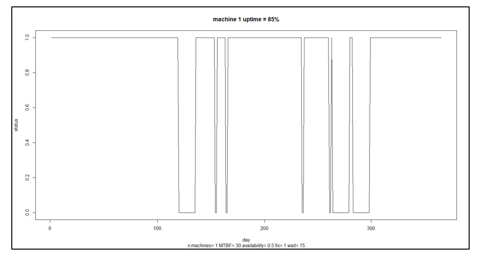
Step 5 can vary depending on the user’s goals. Computing the MTBF is standard. Choose others to suit the problem. Besides the summary statistics provided by step 5, individual simulation runs can be plotted to build intuition about the random dynamics of machine uptime and downtime. Figure 3 shows an example for a single machine showing alternating cycles of uptime and downtime resulting in 85% uptime.

Figure 3 A sample scenario for a single machine

Figure 3 A sample scenario for a single machine


Benefits of Machine Reliability Models

In Figure 3, the machine is up and running 85% of the time. That may not be good enough. You may have some ideas about how to improve the machine’s reliability, e.g., maybe you can improve the reliability of component 3 by buying a newer, better version from a different supplier. How much would that help? That is hard to guess: component 3 may only one of several and perhaps not the weakest link, and how much the change pays off depends on how much better the new one would be. Maybe you should develop a specification for component 3 that you can then shop to potential suppliers, but how long does component 3 have to last to have a material impact on the machine’s MTBF?

This is where having a model pays off. Without a model, you’re relying on guesswork. With a model, you can turn speculation about what-if situations into accurate estimates. For instance, you could analyze how a 10% increase in MTBF for component 3 would translate into an improvement in MTBF for the entire machine.

As another example, suppose you have seven machines producing an important product. You calculate that you must dedicate six of the seven to fill a major order from your one big customer, leaving one machine to handle demand from a number of miscellaneous small customers and to serve as a spare. A reliability model for each machine could be used to estimate the probabilities of various contingencies: all seven machines work and life is good; six machines work so you can at least keep your key customer happy; only five machines work so you have to negotiate something with your key customer, etc.

In sum, probability models of machine or component failure can provide the basis for converting failure time data into smart business decisions.


Read more about  Maximize Machine Uptime with Probabilistic Modeling


Read more about   Probabilistic forecasting for intermittent demand


Leave a Comment
Related Posts
Why MRO Businesses Need Add-on Service Parts Planning & Inventory Software

Why MRO Businesses Need Add-on Service Parts Planning & Inventory Software

MRO organizations exist in a wide range of industries, including public transit, electrical utilities, wastewater, hydro power, aviation, and mining. To get their work done, MRO professionals use Enterprise Asset Management (EAM) and Enterprise Resource Planning (ERP) systems. These systems are designed to do a lot of jobs. Given their features, cost, and extensive implementation requirements, there is an assumption that EAM and ERP systems can do it all. In this post, we summarize the need for add-on software that addresses specialized analytics for inventory optimization, forecasting, and service parts planning.

Head to Head: Which Service Parts Inventory Policy is Best?

Head to Head: Which Service Parts Inventory Policy is Best?

Our customers have usually settled into one way to manage their service parts inventory. The professor in me would like to think that the chosen inventory policy was a reasoned choice among considered alternatives, but more likely it just sort of happened. Maybe the inventory honcho from long ago had a favorite and that choice stuck. Maybe somebody used an EAM or ERP system that offered only one choice. Perhaps there were some guesses made, based on the conditions at the time.

Leveraging ERP Planning BOMs with Smart IP&O to Forecast the Unforecastable

Leveraging ERP Planning BOMs with Smart IP&O to Forecast the Unforecastable

In a highly configurable manufacturing environment, forecasting finished goods can become a complex and daunting task. The number of possible finished products will skyrocket when many components are interchangeable. A traditional MRP would force us to forecast every single finished product which can be unrealistic or even impossible. Several leading ERP solutions introduce the concept of the “Planning BOM”, which allows the use of forecasts at a higher level in the manufacturing process. In this article, we will discuss this functionality in ERP, and how you can take advantage of it with Smart Inventory Planning and Optimization (Smart IP&O) to get ahead of your demand in the face of this complexity.

Call an Audible to Proactively Counter Supply Chain Noise


You know the situation: You work out the best way to manage each inventory item by computing the proper reorder points and replenishment targets, then average demand increases or decreases, or demand volatility changes, or suppliers’ lead times change, or your own costs change. Now your old policies (reorder points, safety stocks, Min/Max levels, etc.)  have been obsoleted – just when you think you’d got them right.   Leveraging advanced planning and inventory optimization software gives you the ability to proactively address ever-changing outside influences on your inventory and demand.  To do so, you’ll need to regularly recalibrate stocking parameters based on ever-changing demand and lead times.

Recently, some potential customers have expressed concern that by regularly modifying inventory control parameters they are introducing “noise” and adding complication to their operations. A visitor to our booth at last week’s Microsoft Dynamics User Group Conference commented:

“We don’t want to jerk around the operations by changing the policies too often and introducing noise into the system. That noise makes the system nervous and causes confusion among the buying team.”

This view is grounded in yesterday’s paradigms.  While you should generally not change an immediate production run, ignoring near-term changes to the policies that drive future production planning and order replenishment will wreak havoc on your operations.   Like it or not, the noise is already there in the form of extreme demand and supply chain variability.  Fixing replenishment parameters, updating them infrequently, or only reviewing at the time of order means that your Supply Chain Operations will only be able to react to problems rather than proactively identify them and take corrective action.

Modifying the policies with near-term recalibrations is adapting to a fluid situation rather than being captive to it.  We can look to this past weekend’s NFL games for a simple analogy. Imagine the quarterback of your favorite team consistently refusing to call an audible (change the play just before the ball is snapped) after seeing the defensive formation.  This would result in lots of missed opportunities, inefficiency, and stalled drives that could cost the team a victory.  What would you want your quarterback to do?

Demand, lead times, costs, and business priorities often change, and as these last 18 months have proved they often change considerably.  As a Supply Chain leader, you have a choice:  keep parameters fixed resulting in lots of knee-jerk expedites and order cancellations, or proactively modify inventory control parameters.  Calling the audible by recalibrating your policies as demand and supply signals change is the right move.

Here is an example. Suppose you are managing a critical item by controlling its reorder point (ROP) at 25 units and its order quantity (OQ) at 48. You may feel like a rock of stability by holding on to those two numbers, but by doing so you may be letting other numbers fluctuate dramatically.  Specifically, your future service levels, fill rates, and operating costs could all be resetting out of sight while you fixate on holding onto yesterday’s ROP and OQ.  When the policy was originally determined, demand was stable and lead times were predictable, yielding service levels of 99% on an important item.   But now demand is increasing and lead times are longer.  Are you really going to expect the same outcome (99% service level) using the same sets of inputs now that demand and lead times are so different?  Of course not.  Suppose you knew that given the recent changes in demand and lead time, in order to achieve the same service level target of 99%, you had to increase the ROP to 35 units.  If you were to keep the ROP at 25 units your service level would fall to 92%.  Is it better to know this in advance or to be forced to react when you are facing stockouts?

What inventory optimization and planning software does is make visible the connections between performance metrics like service rate and control parameters like ROP and ROQ. The invisible becomes visible, allowing you to make reasoned adjustments that keep your metrics where you need them to be by adjusting the control levers available for your use.  Using probabilistic forecasting methods will enable you to generate Key Performance Predictions (KPPs) of performance and costs while identifying near-term corrective actions such as targeted stock movements that help avoid problems and take advantage of opportunities. Not doing so puts your supply chain planning in a straightjacket, much like the quarterback who refuses to audible.

Admittedly, a constantly-changing business environment requires constant vigilance and occasional reaction. But the right inventory optimization and demand forecasting software can recompute your control parameters at scale with a few mouse clicks and clue your ERP system how to keep everything on course despite the constant turbulence.  The noise is already in your system in the form of demand and supply variability.  Will you proactively audible or stick to an older plan and cross your fingers that things will work out fine?


Leave a Comment
Related Posts
Why MRO Businesses Need Add-on Service Parts Planning & Inventory Software

Why MRO Businesses Need Add-on Service Parts Planning & Inventory Software

MRO organizations exist in a wide range of industries, including public transit, electrical utilities, wastewater, hydro power, aviation, and mining. To get their work done, MRO professionals use Enterprise Asset Management (EAM) and Enterprise Resource Planning (ERP) systems. These systems are designed to do a lot of jobs. Given their features, cost, and extensive implementation requirements, there is an assumption that EAM and ERP systems can do it all. In this post, we summarize the need for add-on software that addresses specialized analytics for inventory optimization, forecasting, and service parts planning.

Head to Head: Which Service Parts Inventory Policy is Best?

Head to Head: Which Service Parts Inventory Policy is Best?

Our customers have usually settled into one way to manage their service parts inventory. The professor in me would like to think that the chosen inventory policy was a reasoned choice among considered alternatives, but more likely it just sort of happened. Maybe the inventory honcho from long ago had a favorite and that choice stuck. Maybe somebody used an EAM or ERP system that offered only one choice. Perhaps there were some guesses made, based on the conditions at the time.

Leveraging ERP Planning BOMs with Smart IP&O to Forecast the Unforecastable

Leveraging ERP Planning BOMs with Smart IP&O to Forecast the Unforecastable

In a highly configurable manufacturing environment, forecasting finished goods can become a complex and daunting task. The number of possible finished products will skyrocket when many components are interchangeable. A traditional MRP would force us to forecast every single finished product which can be unrealistic or even impossible. Several leading ERP solutions introduce the concept of the “Planning BOM”, which allows the use of forecasts at a higher level in the manufacturing process. In this article, we will discuss this functionality in ERP, and how you can take advantage of it with Smart Inventory Planning and Optimization (Smart IP&O) to get ahead of your demand in the face of this complexity.