What’s all the hoopla around the term “probabilistic forecasting?” Is it just a more recent marketing term some software vendors and consultants have coined to feign innovation? Is there any real tangible difference compared to predecessor “best fit” techniques?  Aren’t all forecasts probabilistic anyway?

To answer this question, it is helpful to think about what the forecast really is telling you in terms of probabilities.  A “good” forecast should be unbiased and therefore yield a 50/50 probability being higher or lower than the actual.  A “bad” forecast will build in subjective buffers (or artificially depress the forecast) and result in demand that is either biased high or low.  Consider a salesperson that intentionally reduces their forecast by not reporting sales they expect to close to be “conservative.” Their forecasts will have negative forecast bias as actuals will nearly always be higher than what they predicted.   On the other hand, consider a customer that provides an inflated forecast to their manufacturer.  Worried about stockouts, they overestimate demand to ensure their supply.  Their forecast will have a positive bias as actuals will nearly always be lower than what they predicted. 

These types of one-number forecasts described above are problematic.  We refer to these predictions as “point forecasts” since they represent one point (or a series of points over time) on a plot of what might happen in the future.   They don’t provide a complete picture because to make effective business decisions such as determining how much inventory to stock or the number of employees to be available to support demand requires detailed information on how much lower or higher the actual will be!  In other words, you need the probabilities for each possible outcome that might occur.  So, by itself, the point forecast isn’t probabilistic one.   

To get a probabilistic forecast, you need to know the distribution of possible demands around that forecast.  Once you compute this, the forecast becomes “probabilistic.”  How forecasting systems and practitioners such as demand planners, inventory analysts, material managers, and CFOs determine these probabilities is the heart of the question: “what makes a forecast probabilistic?”     

Normal Distributions
Most forecasts and the systems/software that produce them start with a prediction of demand.  Then they figure out the range of possible demands around that forecast by making incorrect theoretical assumptions about the distribution.  If you’ve ever used a “confidence interval” in your forecasting software, this is based on a probability distribution around the forecast.  The way this range of demand is determined is to assume a particular type of distribution.  Most often this means assuming a bell shaped, otherwise known as a normal distribution.  When demand is intermittent, some inventory optimization and demand forecasting systems may assume the demand is Poisson shaped. 

After creating the forecast, the assumed distribution is slapped around the demand forecast and you then have your estimate of probabilities for every possible demand – i.e., a “probabilistic forecast.”  These estimates of demand and associated probabilities can then be used to determine extreme values or anything in between if desired.  The extreme values at the upper percentiles of the distribution (i.e., 92%, 95%, 99%, etc.) are most often used as inputs to inventory control models.  For example, reorder points for critical spare parts in an electrical utility might be planned based on a 99.5% service level or even higher.  While a non-critical service part might be planned at an 85% or 90% service level.

The problem with making assumptions about the distribution is that you’ll get these probabilities wrong.  For example, if the demand isn’t normally distributed but you are forcing a bell shaped/normal curve on the forecast then how can then the probabilities will be incorrect.  Specifically, you might want to know the level of inventory needed to achieve a 99% probability of not running out of stock and the normal distribution will tell you to stock 200 units.  But when compared to the actual demand, you come to find out that 200 units only filled demand entirely in 40/50 observations.  So, instead of getting a 99% service level you only achieved an 80% service level!  This is a gigantic miss resulting from trying to fit a square peg into a round hole.  The miss would have led you to take an incorrect inventory reduction.

Empirically Estimated Distributions are Smart
To produce a smart (read accurate) probabilistic forecast you need to first estimate the distribution of demand empirically without any naïve assumptions about the shape of the distribution.  Smart Software does this by running tens of thousands of simulated demand and lead time scenarios.  Our solution leverages patented techniques that incorporate Monte Carlo simulation, Statistical Bootstrapping, and other methods.  The scenarios are designed to simulate real life uncertainty and randomness of both demand and lead times.  Actual historical observations are utilized as the primary inputs, but the solution will give you the option of simulating from non-observed values as well.  For example, just because 100 units was the peak historical demand, that doesn’t mean you are guaranteed to peak out at 100 in the future.  After the scenarios are done you will know the exact probability for each outcome. The “point” forecast then becomes the center of that distribution.  Each future period over time is expressed in terms of the probability distribution associated with that period.

Leaders in Probabilistic Forecasting
Smart Software, Inc. was the first company to ever introduce statistical bootstrapping as part of a commercially available demand forecasting software system twenty years ago.  We were awarded a US patent at the time for it and named a finalist in the APICS Corporate Awards of Excellence for Technological Innovation.  Our NSF Sponsored research that led to this and other discoveries were instrumental in advancing forecasting and inventory optimization.    We are committed to ongoing innovation, and you can find further information about our most recent patent here.

Belmont, MA, June 2023 – Smart Software, Inc., provider of industry-leading demand forecasting, planning, and inventory optimization solutions, today announced the award of US Patent 11,656,887, “SYSTEM AND METHOD TO SIMULATE DEMAND AND OPTIMIZE CONTROL PARAMETERS FOR A TECHNOLOGY PLATFORM.”

The patent directs “technical solutions for analyzing historical demand data of resources in a technology platform to facilitate management of an automated process in the platform.” One important application is optimization of parts inventories.

Aspects of the invention include: an advanced bootstrap process that converts a single observed time series of item demand into an unlimited number of realistic demand scenarios; a performance prediction process that executes Monte Carlo simulations of a proposed inventory control policy to assess its performance; and a performance improvement process that uses the performance prediction process to automatically explore the space of alternative system designs to identify optimal control parameter values, selecting ones that minimize operating cost while guaranteeing a target level of item availability.

The new analytic technology described in the patent will form the basis for the upcoming release of the next generation (“Gen2”) of Smart Demand Planner™ and Smart IP&O™. Current customers and resellers can preview Gen2 by contacting their Smart Software sales representative.

Research underlying the patent was self-funded by Smart, supplemented by competitive Small Business Innovation Research grants from the US National Science Foundation.

About Smart Software, Inc.
Founded in 1981, Smart Software, Inc. is a leader in providing businesses with enterprise-wide demand forecasting, planning, and inventory optimization solutions.  Smart Software’s demand forecasting and inventory optimization solutions have helped thousands of users worldwide, including customers such as Disney, Arizona Public Service, Ameren, and The American Red Cross.  Smart’s Inventory Planning & Optimization Platform, Smart IP&O gives demand planners the tools to handle sales seasonality, promotions, new and aging products, multi-dimensional hierarchies, and intermittently demanded service parts and capital goods items.  It also provides inventory managers with accurate estimates of the optimal inventory and safety stock required to meet future orders and achieve desired service levels.  Smart Software is headquartered in Belmont, Massachusetts, and our website is www.smartcorp.com.

Many companies looking to improve their forecasting process don’t know where to start. It can be confusing to contend with learning new statistical methods, making sure data is properly structured and updated, agreeing on who “owns” the forecast, defining what ownership means, and measuring accuracy. Having seen this over forty-plus years of practice, we wrote this blog to outline the core focus and to encourage you to keep it simple early on.

1. Objectivity. First, understand and communicate that the Demand Planning and Forecasting process is an exercise in objectivity. The focus is on getting inputs from various sources (stakeholders, customers, functional managers, databases, suppliers, etc.) and deciding whether those inputs add value. For example, if you override a statistical forecast and add 20% to the projection, you should not just assume that you automatically got it right. Instead, be objective and check whether that override increased or decreased forecast accuracy. If you find that your overrides made things worse, you’ve gained something: This informs the process and you know to better scrutinize override decisions in the future.

2.  Teamwork. Recognize that forecasting and demand planning are team sports. Agree on who will captain the team. The captain is responsible for creating the baseline statistical forecasts and supervising the demand planning process. But results depend on everyone on the team making positive contributions, providing data, suggesting alternative methodologies, questioning assumptions, and executing recommended actions. The final results are owned by the company and every single stakeholder.

3. Measurement. Don’t fixate on industry forecast accuracy benchmarks. Every SKU has its own level of “forecastability”, and you may be managing any number of difficult items. Instead, create your own benchmarks based on a sequence of increasingly advanced forecasting methods. Advanced statistical forecasts may seem dauntingly complex at first, so start simple with a basic method, such as forecasting the historical average demand. Then measure how close that simple forecast comes to the actual observed demand. Work up from there to techniques that deal with complications like trend and seasonality. Measure progress using accuracy metrics calculated by your software, such as the mean absolute percentage error (MAPE). This will allow your company to get a little bit better each forecast cycle.

4. Tempo. Then focus efforts on making forecasting a standalone process that isn’t combined with the complex process of inventory optimization. Inventory management is built on a foundation of sound demand forecasting, but it is focused on other topics: what to purchase, when to purchase, minimum order quantities, safety stocks, inventory levels, supplier lead times, etc. Let inventory management go to later. First build up “forecasting muscle” by creating, reviewing, and evolving the forecasting process to have a regular cadence. When your process is sufficiently matured, catch up with the increasing speed of business by increasing the tempo of your forecasting process to at least a monthly cadence.

Remarks

Revising a company’s forecasting process can be a major step. Sometimes it happens when there is executive turnover, sometimes when there is a new ERP system, sometimes when there is new forecasting software. Whatever the precipitating event, this change is an opportunity to rethink and refine whatever process you had before. But trying to eat the whole elephant in one go is a mistake. In this blog, we’ve outlined some discrete steps you can take to make for a successful evolution to a better forecasting process.

Outside of work, you may have heard the famous dictum “Correlation is not causation.” It may sound like a piece of theoretical fluff that, though involved in a recent Noble Prize in economics, isn’t relevant to your work as a demand planner. Is so, you may be only partially correct.

Extrapolative vs Causal Models

Most demand forecasting uses extrapolative models. Also called time-series models, these forecast demand using only the past values of an item’s demand. Plots of past values reveal trend and seasonality and volatility, so there is a lot they are good for. But there is another type of model – causal models —that can potentially improve forecast accuracy beyond what you can get from extrapolative models.

Causal models bring more input data to the forecasting task: information on presumed forecast “drivers” external to the demand history of an item. Examples of potentially useful causal factors include macroeconomic variables like the inflation rate, the rate of GDP growth, and raw material prices. Examples not tied to the national economy include industry-specific growth rates and your own and competitors’ ad spending.  These variables are usually used as inputs to regression models, which are equations with demand as an output and causal variables as inputs.

Forecasting using Causal Models

Many firms have an S&OP process that involves a monthly review of statistical (extrapolative) forecasts in which management adjusts forecasts based on their judgement. Often this is an indirect and subjective way to work causal models into the process without doing the regression modeling.

To actually make a causal regression model, first you have to nominate a list of potentially-useful causal predictor variables. These may come from your subject matter expertise. For example, suppose you manufacture window glass. Much of your glass may end up in new homes and new office buildings. So, the number of new homes and offices being built are plausible predictor variables in a regression equation.

There is a complication here: if you are using the equation to predict something, you must first predict the predictors. For example, sales of glass next quarter may be strongly related to numbers of new homes and new office buildings next quarter. But how many new homes will there be next quarter? That’s its own forecasting problem. So, you have a potentially powerful forecasting model, but you have extra work to do to make it usable.

There is one way to simplify things: if the predictor variables are “lagged” versions of themselves. For example, the number of new building permits issued six months ago may be a good predictor of glass sales next month. You don’t have to predict the building permit data – you just have to look it up.

Is it a causal relationship or just a spurious correlation?

Causal models are the real deal: there is an actual mechanism that relates the predictor variable to the predicted variable. The example of predicting glass sales from building permits is an example.

A correlation relationship is more iffy. There is a statistical association that may or may not provide a solid basis for forecasting. For example, suppose you sell a product that happens to appeal most strongly to Dutch people but you don’t realize this. The Dutch are, on average, the tallest people in Europe. If your sales are increasing and the average height of Europeans is increasing, you might use that relationship to good effect. However, if the proportion of Dutch in the Euro zone is decreasing while the average height is increasing because the mix of men versus women is shifting toward men, what can go wrong? You will expect sales to increase because average height is increasing. But your sales are really mostly to the Dutch, and their relative share of the population is shrinking, so your sales are really going to decrease instead. In this case the association between sales and customer height is a spurious correlation.

How can you tell the difference between true and spurious relationships? The gold standard is to do a rigorous scientific experiment. But you are not likely to be in position to do that. Instead, you have to rely on your personal “mental model” of how your market works. If your hunches are right, then your potential causal models will correlate with demand and causal modeling will pay off for you, either to supplement extrapolative models or to replace them.

Here are examples of forecasting problems that SmartForecasts can solve, along with the kinds of business data representative of each.

Forecasting an item based on its pattern

Given the following six quarterly sales figures, what sales can you expect for the third and fourth quarters of 2023?

Sales by Quarter

SmartForecasts gives you many ways to approach this problem. You can make your own statistical forecasts using any of six different exponential smoothing and moving average methods. Or, like most nontechnical forecasters, you can use the time-saving Automatic command, which has been programmed to automatically select and use the most accurate method for your data. Finally, to incorporate your business judgment into the forecasting process, you can graphically adjust any statistical forecast result using SmartForecasts’ “eyeball” adjustment capabilities.

Forecasting an item based on its relationship to other variables.

Given the following historical relationship between unit sales and the number of sales representatives, what sales levels can you expect when the planned increase in sales staff takes place over the final two quarters of 2023?

Sales and Sales Representatives by Quarter

You can answer a question like this using SmartForecasts’ powerful Regression command, designed specifically to facilitate forecasting applications that require regression analysis solutions. Regression models with an essentially unlimited number of independent/predictor variables are possible, although most useful regression models use only a handful of predictors.

Simultaneously forecasting a number of product items and their total

Given the following total sales for all dress shirts and the distribution of sales by color, what will individual and total sales be over the next six months?

Monthly Dress Shirt Sales by Color

SmartForecasts’ unique Group Forecasting features automatically and simultaneously forecasts closely related time series, such as these items in the same product group. This saves considerable time and provides forecast results not only for the individual items but also for their total. “Eyeball” adjustments at both the item and group levels are easy to make. You can quickly create forecasts for product groups with hundreds or even thousands of items.

Forecasting thousands of items automatically

Given the following record of product demand at the SKU level, what can you expect demand to be over the next six months for each of the 5,000 SKUs?

Monthly Product Demand by SKU (Stock Keeping Unit)

In just a few minutes, SmartForecasts’ powerful Automatic Selection can take a forecasting job of this size, read the product demand data, automatically create statistical forecasts for each SKU, and saves the result. The results are then ready for export to your ERP system leveraging any one of our API-based connectors or via file export.  Once set up, forecasts will automatically be produced each planning cycle without intervention by the user.

Forecasting demand that is most often zero

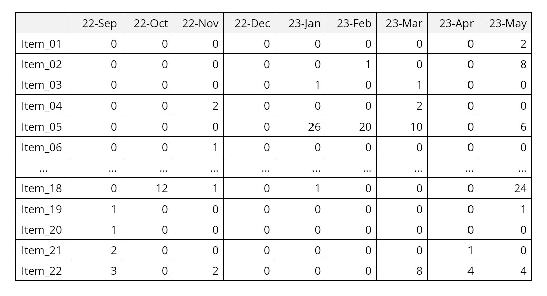
A distinct and especially challenging type of data to forecast is intermittent demand, which is most often zero but jumps up to random nonzero values at random times. This pattern is typical of demand for slow moving items, such as service parts or big ticket capital goods.

For example, consider the following sample of demand for aircraft service parts. Note the preponderance of zero values with nonzero values mixed in, often in bursts.

SmartForecasts has a unique method designed especially for this type of data: the Intermittent Demand forecasting feature. Since intermittent demand arises most often in the context of inventory control, this feature focuses on forecasting the range of likely values for the total demand over a lead time, e.g., cumulative demand over the period Jun-23 to Aug-23 in the example above.

Forecasting inventory requirements

Forecasting inventory requirements is a specialized variant of forecasting that focuses on the high end of the range of possible future values.

For simplicity, consider the problem of forecasting inventory requirements for just one period ahead, say one day ahead. Usually, the forecasting job is to estimate the most likely or average level of product demand. However, if available inventory equals the average demand, there is about a 50% chance that demand will exceed inventory, resulting in lost sales and/or lost good will. Setting the inventory level at, say, ten times the average demand will probably eliminate the problem of stockouts, but will just as surely result in bloated inventory costs.

The trick of inventory optimization is to find a satisfactory balance between having enough inventory to meet most demand without tying up too many resources in the process. Usually, the solution is a blend of business judgment and statistics. The judgmental part is to define an acceptable inventory service level, such as meeting 95% of demand immediately from stock. The statistical part is to estimate the 95th percentile of demand.

When not dealing with intermittent demand, SmartForecasts estimates the required inventory level by assuming a bell-shaped (Normal) curve of demand, estimating both the middle and the width of the bell curve, then using a standard statistical formula to estimate the desired percentile. The difference between the desired inventory level and the average level of demand is called the safety stock because it protects against the possibility of stockouts.

When dealing with intermittent demand, the bell-shaped curve is a poor approximation to the statistical distribution of demand. In this special case, SmartForecasts uses patented intermittent demand forecasting technology to estimate the required inventory service level.