​BACKGROUND

Most of Smart Software’s blogs, webinars and white papers describe the use of our software in “normal operations.” This one is about “irregular operations.”  Smart Software is in the process of adapting our products to help you cope with your own irregular ops. This is a preview.

I first heard the term “irregular operations” when serving a sabbatical tour at the U.S. Federal Aviation Administration in Washington, DC. The FAA abbreviates the term to “IROPS” and uses it to describe situations in which weather, mechanical problems or other issues disrupt the normal flow of aircraft.

Smart Inventory Optimization® (“SIO”) currently works to provide what are known as “steady state” policies for managing inventory items. That means, for instance, that SIO automatically calculates values for reorder points (ROP’s) and order quantities (OQ’s) that are meant to last for the foreseeable future. It computes these values based on simulations of daily operations that extend years into the future. If and when the unforeseeable happens, our regime change detection method reacts by removing obsolete data and allowing recalculation of the ROP’s and OQ’s.

We often note the increasing speed of business, which shortens the duration of the “foreseeable future.” Some of our customers are now adopting shorter planning horizons, such as moving from quarterly to monthly plans. One side effect of this change is that IROPS have become more consequential. If a plan is based on three simulated years of daily demand, one odd event, like a large surprise order, doesn’t matter much in the grand scheme of things. But if the planning horizon is very short, one big surprise demand can have a major effect on key performance indicators (KPI’s) computed over a shorter interval – there is no time for “averaging out”. The planner may be forced to place an emergency replenishment order to deal with the disruption. When should the order be placed to do the most good? How big should it be?

SCENARIO: NORMAL OPS

To make this concrete, consider the following scenario. Tom’s Spares, Inc. provides critical service parts to its customers, including SKU723, a replacement circuit board sold under the trade name WIDGET. Demand for WIDGET is intermittent, with less than one unit demanded per day. Tom’s Spares orders WIDGETs from Acme Products, who take either 7 or 10 days to fulfill replenishment orders.

Tom’s Spares operates with a short inventory planning horizon of 28 days. The company operates in a competitive environment with impatient customers who only grudgingly accept backorders. Tom’s policy is to set ROP’s and OQ’s to keep inventory lean while maintaining a fill rate of at least 90%. Management monitors KPI’s on a monthly basis. In the case of WIDGETS, these KPI targets are currently met using an ROP=3 and an OQ=4, resulting in an average on hand of about 4 units and average fill rate of 96%.  Tom’s Spares has a pretty good thing going for WIDGETS.

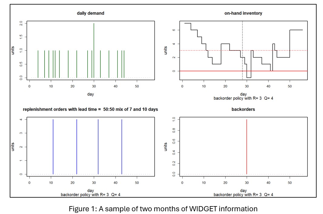
Figure 1 shows two months of WIDGET information. The top left panel shows daily unit demand. The top right shows daily units on hand. The bottom left panel shows the timing and size of replenishment orders back to Acme Products. The bottom right shows units backordered due to stockouts. In this simulation, daily demand was either 0 or 1, with one demand of 2 units. On hand units began the month at 7 and never dropped below 1, though in the next month there was a stockout resulting in a single unit on backorder. Over the two months, there were 4 replenishment orders of 4 units each sent to Acme, all of which arrived during the two-month simulation period.

GOOD TROUBLE DISRUPTS NORMAL OPS

Now we add some “good trouble” to the scenario: An unusually large order arises part way through the planning period. It’s “good” because more demand implies more revenue. But it’s “trouble” because the normal ops inventory control parameters (ROP=3, OQ=4) were not chosen to cope with this situation. The spike in demand might be so big, and so disadvantageously timed, as to overwhelm the inventory system, creating stockouts and their attendant backorders. The KPI report to management for such a month would not be pretty.

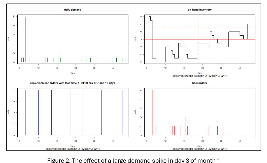
Figure 2 shows a scenario in which a demand spike of 10 units hits in the third day of the planning period. In this case, the spike puts the inventory under water for the rest of the month and creates a cascade of backorders extending into the next month. Averaging over 1,000 simulations, month 1 KPI’s show an average on hand of 0.6 units and a miserable 44% fill rate.

FIGHTING BACK WITH IRREGULAR OPERATIONS

Tom’s Spares can respond to an irregular situation with an irregular move by creating an emergency replenishment order. To do it right, they have to think about (a) when to place the order (b) how big the order should be and (c) whether to expedite the order.

The timing question seems obvious: react as soon as the order hits. However, if the customer were to provide early warning, Tom’s Spares could order early and be in better position to limit the disruption from the spike. However, if communication between Tom’s and the customer making the big order is spotty, then the customer might give Tom’s a heads-up later or not at all.

The size of the special order seems obvious too: pre-order the required number of units. But that works best if Tom’s Spares knows when the demand spike will hit. If not, it might be a good idea to order extra to limit the duration of any backorders. In general, the less early warning provided, the larger the order Tom’s should make. This relationship could be explored with simulation, of course.

The arrival of the replenishment order could be left to the usual operation of Acme Products. In the simulations above, Acme was equally likely to respond in 7 or 14 days. For a 28-day planning horizon, taking a risk on getting a 14-day response might be asking for trouble, so it may be especially worthwhile for Tom’s to pay Acme for expedited shipping. Maybe overnight, but possibly something cheaper but still relatively fast.

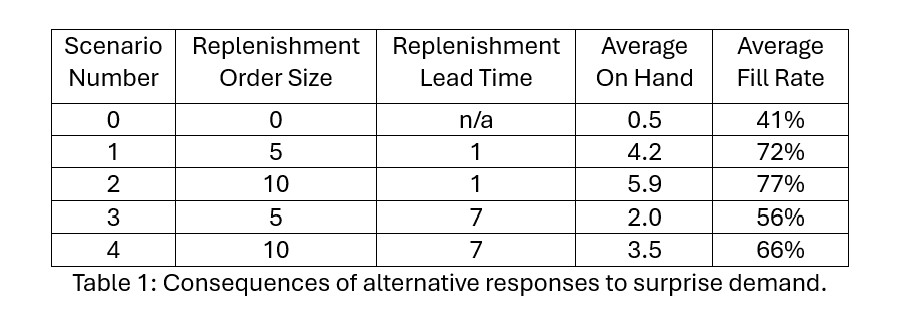
We explored a few more scenarios using simulation. Table 1 shows the results. Scenarios 1-4 assume a surprise additional demand of 10 units arrives on Day 3, triggering an immediate order for  additional replenishment. The size and lead time of the replenishment order varies.

Scenario 0 shows that doing nothing in response to the surprise demand leads to an abysmal 41% fill rate for that month; not shown is that this result sets of the next month for continued poor performance. Regular operations won’t do well. The planner must do something to respond to the anomalous demand.

Doing something in response involves making a one-time emergency replenishment order. The planner must choose the size and timing of that order. Scenarios 1 and 3 depict “half sized” replenishments. Scenarios 1 and 2 depict overnight replenishments, while scenarios 3 and 4 depict guaranteed one week response.

The results make clear that immediate response is more important than the size of the replenishment order for restoring the Fill Rate. Overnight replenishment produces fill rates in the 70% range, while one-week replenishment lead time drops the fill rate into the mid-50% to mid-60% range.

TAKEAWAYS

Inventory management software is expanding from its traditional focus on normal ops to an additional focus on irregular ops (IROPS). This evolution has been made possible by the development of new statistical methods for generating demand scenarios at a daily level.

We considered one IROPS situation: surprise arrival of an anomalously large demand. Daily simulations provided guidance about the timing and size of an emergency replenishment order. Results from such an analysis provide inventory planners with critical backup by estimating the results of alternative interventions that their experience suggests to them.

This video blog holds essential insights for those working with the complexities of inventory management. The session focuses on striking the right balance within the inventory tradeoff curve, inviting viewers to understand the deep-seated importance of this equilibrium. If you’ve ever had to manage stock, you’ll know it feels like a bit of a tug-of-war. On one side, you’re pulling towards less inventory, which is great for saving money but can leave your customers high and dry. On the other, you’re considering more inventory, which keeps your customers happy but can be a pain for your budget. To make a smart choice in this ongoing tug-of-war, you need to understand where your current inventory decisions place you on this tradeoff curve. Are you at a point where you can handle the pressure, or do you need to shuffle along to a more comfortable spot?

If you can’t answer this question, it means that you still rely on outdated methods, risking the potential for surplus inventory or unmet customer needs. Watch the video so you can see exactly where you are on this curve and understand better about whether you want to stay put or move to a more optimal position.

And if you decide to move, we’ve got the tools to guide you. Smart IP&O’s advanced “what-if” analysis enables businesses to precisely evaluate the impact of different inventory strategies, such as adjustments to safety stock levels or changes in reorder points, on their balance between holding costs and service levels. By simulating demand scenarios and inventory policies, Smart IP&O provides a clear visualization of potential financial outcomes and service level implications, allowing for data-driven strategic decisions. This powerful tool ensures businesses can achieve an optimal balance, minimizing excess inventory and related costs while maintaining high service levels to meet customer demand efficiently.  

​In this video blog, we explore the critical roles of Descriptive, Predictive, and Prescriptive Analytics in inventory management, highlighting their essential contributions to driving supply chain optimization through strategic foresight and insightful data analysis.

​These analytics foster a dynamic, responsive, and efficient inventory management ecosystem by enabling inventory managers to monitor current operations, anticipate future developments, and formulate optimal responses. We’ll walk you through how Descriptive Analytics keeps you informed about current operations, Predictive Analytics helps you anticipate future demands, and Prescriptive Analytics guides your strategic decisions for maximum efficiency and cost-effectiveness.

By the end of the video, you’ll have a solid understanding of how to leverage these analytics to enhance your inventory management strategies. These are not just tools but a new way of thinking about and approaching inventory optimization with the support of modern software.

Our customers have usually settled into one way to manage their service parts inventory. The professor in me would like to think that the chosen inventory policy was a reasoned choice among considered alternatives, but more likely it just sort of happened. Maybe the inventory honcho from long ago had a favorite and that choice stuck. Maybe somebody used an EAM or ERP system that offered only one choice. Perhaps there were some guesses made, based on the conditions at the time.

The Competitors

Too seldom, businesses make these choices in haphazard ways. But modern service parts planning software lets you be more systematic about your choices. This post demonstrates that proposition by making objective comparisons among three popular inventory policies:  Order Up To, Reorder Point/Order Quantity, and Min/Max.  I discussed each of these policies in this video blog.

• Order Up To. This is a periodic review policy where every T days, on-hand inventory is tallied and an order of random size is placed to bring the stock level back up to S units.
• Q, R or Reorder Point/Order Quantity. Q, R is a continuous review policy where every day, inventory is tallied. If there are Q or fewer units on hand, an order of fixed size is placed for R more units.
• Min, Max is another continuous review policy where every day, inventory is tallied. If there are Min or fewer units on hand, an order is placed to bring the stock level back up to Max units.

Inventory theory says these choices are listed in increasing order of effectiveness. The first option, Order Up To, is clearly the simplest and cheapest to implement, but it closes its eyes to what’s going on for long periods of time.  Imposing a specified passage of time in between orders makes it, in theory, less flexible. In contrast, the two continuous review options keep an eye on what’s happening all the time, so they can react to potential stockouts quicker. The Min/Max option is, in theory, more flexible than the option that uses a fixed reorder quantity because the size of the order dynamically changes to accommodate the demand.

That’s the theory. This post examines evidence from head-to-head comparisons to check the theory and put concrete numbers on the relative performance of the three policies.

The Meaning of “Best”

How should we keep score in this tournament? If you are a regular reader of this Smart Forecaster blog, you know that the core of inventory planning is a tug-of-war between two opposing objectives: keeping inventory lean vs keeping item availability metrics such as service level high.

To simplify things, we will compute “one number to rule them all”: the average operating cost. The winning policy will be the one with the lowest average.

This average is the sum of three components: the cost of holding inventory (“holding cost”), the cost of ordering replenishment units (“ordering cost”) and the cost of losing a sale (“shortage cost”). To make things concrete, we used the following assumptions:

• Each service part is valued at $1,000.
• Annual holding cost is 10% of item value, or $100 per year per unit.
• Processing each replenishment order costs $20 per order.
• Each unit demanded but not provided costs the value of the part, $1,000.

For simplicity, we will refer to the average operating cost as simply “the cost”.

Of course, the lowest average cost can be achieved by getting out of the business. So the competition required a performance constraint on item availability: Each option had to achieve a fill rate of at least 99%.

The Alternatives Duke it Out

A key element of context is whether stockouts result in losses or backorders. Assuming that the service part in question is critical, we assumed that unfilled orders are lost, which means that a competitor fills the order. In an MRO environment, this will mean additional downtime due to stockout.

To compare the alternatives, we used our predictive modeling engine to run a large number of Monte Carlo simulations.  Each simulation involved specifying the parameter values of each policy (e.g., Min and Max values), generating a demand scenario, feeding that into the logic of the policy, and measuring the resulting cost averaged over 365 days of operation. Repeating this process 1,000 times and averaging the 1,000 resulting costs gave the final result for each policy.  

To make the comparison fair, each alternative had to be designed for its best performance. So we searched the “design space” of each policy to find the design with the lowest cost. This required repeating the process described in the previous paragraph for many pairs of parameter values and identifying the pair yielding the lost average annual operating cost.

Using the algorithms in Smart Inventory Optimization (SIO^TM) we made head-to-head-to-head comparisons under the following assumptions about demand and supply:

• Item demand was assumed to be intermittent and highly variable but relatively simple in that there was neither trend nor seasonality, as is often true for service parts. Daily mean demand was 5 units with a large standard deviation of 13 units. Figure 1 shows a sample of one year’s demand. We have chosen a very challenging demand pattern, in which some days have 10 to even 20 times the average demand.

Figure 1: Daily part demand was assumed to be intermittent and very spikey.

​​

• Suppliers’ replenishment lead times were 14 days 75% of the time and 21 days otherwise. This reflects the fact that there is always uncertainty in the supply chain.

And the Winner Is…

Was the theory right? Kinda’ sorta’.

Table 1 shows the results of the simulation experiments. For each of the three competing policies, it shows the average annual operating cost, the margin of error (technically, an approximate 95% confidence interval for the mean cost), and the apparent best choices for parameter values.

Table 1: Results of the simulated comparisons

For example, the average cost for the (T,S) policy when T is fixed at 30 days was $41,680. But the Plus/Minus implies that the results are compatible with a “true” cost (i.e., the estimate from an infinite number of simulations) of anywhere between $39,890 and $43,650. The reason there is so much statistical uncertainty is the extremely spikey nature of demand in this example.

Table 1 says that, in this example, the three policies fall in line with expectations. However, more useful conclusions would be:

1. The three policies are remarkably similar in average cost. By clever choice of parameter values, one can get good results out of any of the three policies.
2. Not shown in Table 1, but clear from the detailed simulation results, is that poor choices for parameter values can be disastrous for any policy.
3. It is worth noting that the periodic review (T,S) policy was not allowed to optimize over possible values of T. We fixed T at 30 to mimic what is common in practice, but those who use the periodic review policy should consider other review periods. An additional experiment fixed the review period at T = 7 days. The average cost in this scenario was minimized at $36,551 ± $1,668 with S = 343. This result is better than that using T = 30 days.
4. We should be careful about over-generalizing these results. They depend on the assumed values of the three cost parameters (holding, ordering and shortage) and the character of the demand process.
5. It is possible to run experiments like those shown here automatically in Smart Inventory Optimization. This means that you too would be able to explore design choices in a rigorous way.

In this article, we will review the “suggested orders” functionality in Epicor BisTrack, explain its limitations, and summarize how Smart Inventory Planning & Optimization (Smart IP&O) can help reduce inventory & minimize stock-outs by accurately assessing the tradeoffs between stockout risks and inventory costs.

Automating Replenishment in Epicor BisTrack
Epicor BisTrack’s “Suggested Ordering” can manage replenishment by suggesting what to order and when via reorder point-based policies such as min-max and/or manually specified weeks of supply. BisTrack contains some basic functionality to compute these parameters based on average usage or sales, supplier lead time, and/or user-defined seasonal adjustments. Alternatively, reorder points can be specified completely manually. BisTrack will then present the user with a list of suggested orders by reconciling incoming supply, current on hand, outgoing demand, and stocking policies.

How Epicor BisTrack “Suggested Ordering” Works
To get a list of suggested orders, users specify the methods behind the suggestions, including locations for which to place orders and how to determine the inventory policies that govern when a suggestion is made and in what quantity.

First, the “method” field is specified from the following options to determine what kind of suggestion is generated and for which location(s):

Purchase – Generate purchase order recommendations.

1. Centralized for all branches – Generates suggestions for a single location that buys for all other locations.
2. By individual branch – Generates suggestions for multiple locations (vendors would ship directly to each branch).
3. By source branch – Generates suggestions for a source branch that will transfer material to branches that it services (“hub and spoke”).
4. Individual branches with transfers – Generates suggestions for an individual branch that will transfer material to branches that it services (“hub and spoke”, where the “hub” does not need to be a source branch).

Manufacture – Generate work order suggestions for manufactured goods.

1. By manufacture branch.
2. By individual branch.

Transfer from source branch – Generate transfer suggestions from a given branch to other branches.

Next, the “suggest order to” is specified from the following options:

1. Minimum – Suggests orders “up to” the minimum on hand quantity (“min”). For any item where supply is less than the min, BisTrack will suggest an order suggestion to replenish up to this quantity.
2. Maximum when less than min – Suggests orders “up to” a maximum on-hand quantity when the minimum on-hand quantity is breached (e.g. a min-max inventory policy).

3. Based on cover (usage) – Suggests orders based on coverage for a user-defined number of weeks of supply with respect to a specified lead time. Given internal usage as demand, BisTrack will recommend orders where supply is less than the desired coverage to cover the difference.

4. Based on over (sales) – Suggests orders based on coverage for a user-defined number of weeks of supply with respect to a specified lead time. Given sales orders as demand, BisTrack will recommend orders where supply is less than the desired coverage to cover the difference.

5. Maximum only – Suggests orders “up to” a maximum on-hand quantity where supply is less than this max.

Finally, if allowing BisTrack to determine the reorder thresholds, users can specify additional inventory coverage as buffer stock, lead times, how many months of historical demand to consider, and can also manually define period-by-period weighting schemes to approximate seasonality. The user will be handed a list of suggested orders based on the defined criteria. A buyer can then generate POs for suppliers with the click of a button.

Limitations

Rule-of-thumb Methods

While BisTrack enables organizations to generate reorder points automatically, these methods rely on simple averages that do not capture seasonality, trends, or the volatility in an item’s demand. Averages will always lag behind these patterns and are unable to pick up on trends. Consider a highly seasonal product like a snow shovel—if we take an average of Summer/Fall demand as we approach the Winter season instead of looking ahead, then the recommendations will be based on the slower periods instead of anticipating upcoming demand. Even if we consider an entire years’ worth of history or more, the recommendations will overcompensate during the slower months and underestimate the busy season without manual intervention.

Rule of thumb methods also fail when used to buffer against supply and demand variability.  For example, the average demand over the lead time might be 20 units.  However, a planner would often want to stock more than 20 units to avoid stocking out if lead times are longer than expected or demand is higher than the average.  BisTrack allows users to specify the reorder points based on multiples of the averages.  However, because the multiples don’t account for the level of predictability and variability in the demand, you’ll always overstock predictable items and understock unpredictable ones.   Read this article to learn more about why multiples of the average fail when it comes to developing the right reorder point.

Manual Entry
Speaking of seasonality referenced earlier, BisTrack does allow the user to approximate it through the use of manually entered “weights” for each period. This forces the user to have to decide what that seasonal pattern looks like—for every item. Even beyond that, the user must dictate how many extra weeks of supply to carry to buffer against stockouts, and must specify what lead time to plan around. Is 2 weeks extra supply enough? Is 3 enough? Or is that too much? There is no way to know without guessing, and what makes sense for one item might not be the right approach for all items.

Intermittent Demand
Many BisTrack customers may consider certain items “unforecastable” because of the intermittent or “lumpy” nature of their demand. In other words, items that are characterized by sporadic demand, large spikes in demand, and periods of little or no demand at all. Traditional methods—and rule-of-thumb approaches especially—won’t work for these kinds of items. For example, 2 extra weeks of supply for a highly predictable, stable item might be way too much; for an item with highly volatile demand, this same rule might not be enough. Without a reliable way to objectively assess this volatility for each item, buyers are left guessing when to buy and how much.

Reverting to Spreadsheets
The reality is most BisTrack users tend to do the bulk of their planning off-line, in Excel. Spreadsheets aren’t purpose-built for forecasting and inventory optimization. Users will often bake in user-defined rule of thumb methods that often do more harm than good.  Once calculated, users must input the information back into BisTrack manually. The time consuming nature of the process leads companies to infrequently compute their inventory policies – Many months and on occasion years go by in between mass updates leading to a “set it and forget it” reactive approach, where the only time a buyer/planner reviews inventory policy is at the time of order.  When policies are reviewed after the order point is already breached, it is too late.  When the order point is deemed too high, manual interrogation is required to review history, calculate forecasts, assess buffer positions, and to recalibrate.  The sheer volume of orders means that buyers will just release orders rather than take the painstaking time to review everything, leading to significant excess stock.  If the reorder point is too low, it’s already too late.  An expedite may now be required, driving up costs, assuming the customer doesn’t simply go elsewhere.

Epicor is Smarter
Epicor has partnered with Smart Software and offers Smart IP&O as a cross platform add-on to its ERP solutions including BisTrack, a speciality ERP for the Lumber, hardware, and building material industry.  The Smart IP&O solution comes complete with a bidirectional integration to BisTrack.  This enables Epicor customers to leverage built-for-purpose best of breed inventory optimization applications.  With Epicor Smart IP&O you can generate forecasts that capture trend and seasonality without manual configurations.  You will be able to automatically recalibrate inventory policies using field proven, cutting-edge statistical and probabilistic models that were engineered to accurately plan for intermittent demand.   Safety stocks will accurately account for demand and supply variability, business conditions, and priorities.  You can leverage service level driven planning so you have just enough stock or turn on optimization methods that prescribe the most profitable stocking policies and service levels that consider the real cost of carrying inventory. You can support commodity buys with accurate demand forecasting over longer horizons, and run “what-if” scenarios to assess alternative strategies before execution of the plan.

Smart IP&O customers routinely realize 7 figure annual returns from reduced expedites, increased sales, and less excess stock, all the while gaining a competitive edge by differentiating themselves on improved customer service. To see a recorded webinar hosted by the Epicor Users Group that profiles Smart’s Demand Planning and Inventory Optimization platform, please register here.