​​In a highly configurable manufacturing environment, forecasting finished goods can become a complex and daunting task. The number of possible finished products skyrockets when many components are interchangeable. A traditional MRP would force us to forecast every single finished product, which can be unrealistic or even impossible. Several leading solutions introduce the concept of the “Planning BOM,” which allows the use of forecasts at a higher level in the manufacturing process. In this article, we will discuss this functionality in Epicor Kinetic and how you can take advantage of it with Epicor Smart Inventory Planning and Optimization (Smart IP&O) to get ahead of your demand in the face of this complexity.

Why Would I Need a Planning BOM?

Traditionally, each finished product or SKU would have a rigidly defined bill of materials. If we stock that product and want to plan around forecasted demand, we will forecast demand for those products and then feed MRP to blow this forecasted demand from the finished good level down to its components via the BOM.

Many companies, however, offer highly configurable products where customers can select options on the product they buy. As an example, recall the last time you bought a cellphone. You chose a brand and model, but from there, you were likely presented with options: what screen size do you want? How much storage do you want? What color do you prefer? If that business wants to have these cellphones ready and available to ship to you in a reasonable time, suddenly, they are no longer just anticipating demand for that model—they must forecast that model for every type of screen size, for all storage capacities, for all colors, and all possible combinations of those as well! For some manufacturers, these configurations can compound to hundreds or thousands of possible finished good permutations.

There may be so many possible customizations that the demand at the finished product level is completely unforecastable in a traditional sense. Thousands of those cellphones may sell every year, but for each possible configuration, the demand may be extremely low and sporadic—perhaps certain combinations sell once and never again.

This often forces these companies to plan reorder points and safety stock levels mostly at the component level, while largely reacting to firm demand at the finished good level via MRP. While this is a valid approach, it lacks a systematic way to leverage forecasts that may account for anticipated future activity such as promotions, upcoming projects, or sales opportunities. Forecasting at the “configured” level is effectively impossible, and trying to weave in these forecast assumptions at the component level isn’t feasible either.

Planning BOM Explained This is where Planning BOMs come in. Perhaps the sales team is working on a big B2B opportunity for that model, or there’s a planned promotion for Cyber Monday. While trying to work in those assumptions for every possible configuration isn’t realistic, doing it at the model level is totally doable—and tremendously valuable.

The Planning BOM can use a forecast at a higher level and then blow demand down based on predefined proportions for its possible components. For example, the cellphone manufacturer may know that most people opt for 128GB of storage, and far fewer opt for upgrades to 256GB or 512GB. The planning BOM allows the organization to (for example) blow 60% of the demand down to the 128GB option, 30% to the 256GB option, and 10% to the 512GB option. They could do the same for screen sizes, colors, or other available customizations.

The business can now focus its forecast at this model level, leaving the Planning BOM to determine the component mix. Clearly, defining these proportions requires some thought, but Planning BOMs effectively allows businesses to forecast what would otherwise be unforecastable.

The Importance of a Good Forecast

Of course, we still need a good forecast to load into Epicor Kinetic. As explained in this article, while Epicor Kinetic can import a forecast, it often cannot generate one, and when it does it tends to require a great deal of hard-to-use configurations that don’t often get revisited, resulting in inaccurate forecasts. It is, therefore, up to the business to come up with its own sets of forecasts, often manually produced in Excel. Forecasting manually generally presents a number of challenges, including but not limited to:

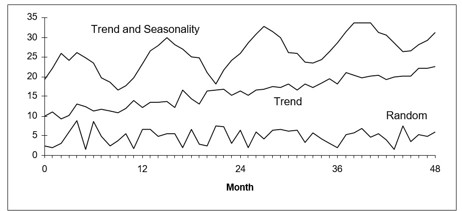
• The inability to identify demand patterns like seasonality or trend.
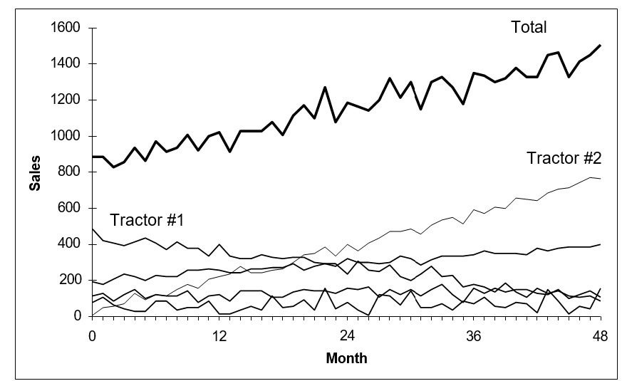
• Overreliance on customer or sales forecasts.
• Lack of accuracy or performance tracking.

No matter how well configured the MRP is with your carefully considered Planning BOMs, a poor forecast means poor MRP output and mistrust in the system—garbage in, garbage out. Continuing along with the “cellphone company” example, without a systematic way of capturing key demand patterns and/or domain knowledge in the forecast, MRP can never see it.

Smart IP&O: A Comprehensive Solution

Smart IP&O supports planning at all levels of your BOM, though the “blowing out” is handled via MRP inside Epicor Kinetic. Here is the method we use for our Epicor Kinetic customers, which is straightforward and effective:

• Smart Demand Planner: The platform contains a purpose-built forecasting application called Smart Demand Planner that you will use to forecast demand for your manufactured products (usually finished goods). It generates statistical forecasts, enables planners to make adjustments and/or weave in other forecasts (such as sales or customer forecasts), and tracks accuracy. The output of this is a forecast that goes into forecast entry inside Epicor Kinetic, where MRP will pick it up. MRP will subsequently use demand at the finished good level, and also blow out material requirements through the BOM, so that demand is recognized at lower levels as well.
• Smart Inventory Optimization: You simultaneously use Smart Inventory Optimization to set min/max/safety levels both for any finished goods you make to stock (if applicable; some of our customers operate purely make-to-order off of firm demand), as well as for raw materials. The key here is that at the raw material level, Smart will leverage job usage demand, supplier lead times, etc., to optimize these parameters while at the same time using sales orders/shipments as demand at the finished good level. Smart handles these multiple inputs of demand elegantly via the bidirectional integration with Epicor Kinetic.

When MRP runs, it nets out supply & demand (which, once again, includes raw material demand blown out from the finished good forecast) against the min/max/safety levels you have established to suggest PO and job suggestions.

Extend Epicor Kinetic with Smart IP&O

Smart IP&O is designed to extend your Epicor Kinetic system with many integrated demand planning and inventory optimization solutions. For example, it can generate statistical forecasts automatically for large numbers of items, allows for intuitive forecast adjustments, tracks forecast accuracy, and ultimately allows you to generate true consensus-based forecasts to better anticipate the needs of your customers.

Thanks to highly flexible product hierarchies, Smart IP&O is perfectly suited to forecasting at the Planning BOM level, so you can capture key patterns and incorporate business knowledge at the levels that matter most. Furthermore, you can analyze and deploy optimal safety stock levels at any level of your BOM.

Leveraging Epicor Kinetic’s Planning BOM capabilities alongside Smart IP&O’s advanced forecasting and inventory optimization features ensures that you can meet demand efficiently and accurately, regardless of the complexity of your product configurations. This synergy not only enhances forecast accuracy but also strengthens overall operational efficiency, helping you stay ahead in a competitive market.

We believe the leading edge of supply chain analytics to be the development of digital twins of inventory systems. These twins take the form of discrete event models that use Monte Carlo simulation to generate and optimize over the full range of operational risks. We also assert that we and our colleagues at Smart Software have played an outsized role in forging that leading edge. But we are not alone: there are a small number of other software firms around the globe who are catching up.

So, what’s next for supply chain analytics? Where is the next frontier? It might involve some sort of neural network model of a distribution system. But we’d give better odds on an extension of our leading-edge models of “single echelon” inventory systems to “multi-echelon” inventory systems.

Figures 1 and 2 illustrate the distinction between single and multiple echelon systems. Figure 1 depicts a manufacturer that relies on a Source to replenish its stock of spare parts or components. When stockouts loom, the manufacturer orders replenishment stock from the Source.

Figure 1: A single-echelon inventory system

Single echelon models do not explicitly include details of the Source. It remains mysterious, an invisible ghost whose only relevant feature is the random time it takes to respond to a replenishment request. Importantly, the Source is implicitly assumed to never itself stock out. That assumption may be “good enough” for many purposes, but it cannot be literally true. It gets handled by stuffing supplier stockout events into the replenishment lead time distribution. Pushing back on that assumption is the rationale for multiechelon modeling.

Figure 2 depicts a simple two-echelon inventory system. It shifts domains from manufacturing to distribution. There are multiple warehouses (WH’s) dependent on a distribution center (DC) for resupply. Now the DC is an explicit part of the model. It has a finite capacity to process orders and requires its own reordering protocols. The DC gets its replenishment from higher up the chain from a Source. The Source might be the manufacturer of the inventory item or perhaps a “regional DC” or something similar, but – guess what? – it is another ghost. As in the single-echelon model, this ghost has one visible characteristic: the probability distribution of its replenishment lead time. (The punch line of a famous joke in physics is “But madame, it’s turtles all the way down.” In our case, “It’s ghosts all the way up.”)

Figure 2: A two-echelon inventory system

The problem of process design and optimization is much harder with two levels. The difficulty is not just the addition of two more control parameters for every WH (e.g., a Min and a Max for each) plus the same two parameters for the DC. Rather, the tougher part is modeling the interaction among the WH’s. In the single-level model, each WH operates in its own little world and never hears “Sorry, we’re stocked out” from the ghostly Source. But in a two-level system, there are multiple WH’s all competing for resupply from their shared DC. This competition creates the main analytical difficulty: the WH’s cannot be modeled in isolation but must be analyzed simultaneously. For instance, if one DC services ten WH’s, there are 2+10×2 = 22 inventory control parameters whose values need to be calculated. In nerd-speak: It is not trivial to solve a 22-variable constrained discrete optimization problem having a stochastic objective function.

If we choose the wrong system design, we discover a new phenomenon inherent in multi-echelon systems, which we informally call “meltdown” or “catastrophe.” In this phenomenon, the DC cannot keep up with the replenishment demands of the WH’s, so it eventually creates stockouts at the warehouse level. Then the WH’s increasingly frantic replenishment requests exhaust the inventory at the DC, which starts its own panicked requests for replenishment from the regional DC. If the regional DC takes too long to refill the DC, then the whole system dissolves into a stockout tragedy.

One solution to the meltdown problem is to overdesign the DC so it almost never runs out, but that can be very expensive, which is why there is a regional DC in the first place. So any affordable system design has a DC that is just good enough to last a long time between meltdowns. This perspective implies a new type of key performance indicator (KPI), such as “Probability of Meltdown within X years is less than Y percent.”

The next frontier will require new methods and new metrics but will offer a new way to design and optimize distribution systems. Our skunk works is already generating prototypes. Watch this space.

In this blog, we will discuss today’s fast-paced and unpredictable market and the constant challenges businesses face in managing their inventory and service levels efficiently. The main subject of this discussion, rooted in the concept of “Probabilistic Inventory Optimization,” focuses on how modern technology can be leveraged to achieve optimal service and inventory targets amidst uncertainty. This approach not only addresses traditional inventory management issues but also offers a strategic edge in navigating the complexities of demand fluctuations and supply chain disruptions.

Understanding and implementing inventory optimization technology is important for several reasons. First, it directly impacts a company’s ability to meet customer demands promptly, thereby affecting customer satisfaction and loyalty. Second, effective inventory management controls operational costs, reducing unnecessary stock holding and minimizing the risk of stockouts or overstocking. In an era where market conditions change rapidly, having a robust system to manage these aspects can be the difference between thriving and merely surviving.

At the heart of inventory management lies a paradox: the need to be prepared for fluctuating demand without succumbing to the pitfalls of overstocking, which can lead to increased holding costs, obsolescence, and wasted resources. Conversely, understocking can result in stockouts, lost sales, and diminished customer satisfaction, ultimately impacting a company’s reputation and bottom line. The unpredictable nature of market demands, compounded by potential supply chain disruptions and changing consumer behavior, adds complexity to this balancing act.

Technology plays a pivotal role here. Modern inventory optimization software integrates probabilistic models, sophisticated forecasting algorithms, and simulation capabilities. These systems help companies respond swiftly to changing market conditions. Furthermore, adopting such technology fosters a culture of data-driven decision-making, ensuring businesses are not merely reacting to uncertainties but proactively strategizing to mitigate their impacts.

Here are brief discussions of the relevant algorithmic technologies.

Probabilistic Inventory Optimization: Traditional inventory management approaches rely on deterministic models that assume a static, predictable world. These models falter in the face of variability and uncertainty. Enter probabilistic inventory optimization, a paradigm that embraces the randomness inherent in supply chain processes. This approach employs statistical models to represent the uncertainties in demand and supply, enabling businesses to account for a full range of possible outcomes.

Advanced Forecasting:  A cornerstone of effective inventory optimization is the ability to anticipate future demand accurately. Advanced forecasting techniques, such as [we don’t sell this outside of SmartForecasts or maybe not even there anymore, so don’t mention it], time series analysis, and machine learning, extract exploitable patterns from historical data.

Safety Stock Calculation: A Shield Against Uncertainty:

Forecasts that include estimates of their own uncertainty enable safety stock calculations. Safety stock acts as a buffer against the unpredictability of demand and supply lead times. Determining the optimal level of safety stock is a critical challenge that probabilistic models address adeptly. With the right safety stock levels, businesses can maintain high service levels, ensuring product availability without the burden of excessive inventory.

Scenario Planning: Preparing for Multiple Futures:

The future is inherently uncertain, and a single forecast can never capture all possible scenarios. Advanced methods that create a range of realistic demand scenarios are the essential form of probabilistic inventory optimization. These techniques allow businesses to explore the implications of multiple futures, from best-case to worst-case situations. By planning against these scenarios, companies can enhance their resilience in the face of market volatility.

Navigating the Future with Confidence

The uncertain landscape of today’s business environment necessitates a shift from traditional inventory management practices to more sophisticated, probabilistic approaches. By embracing the principles of probabilistic inventory optimization, companies can strike a durable balance between service excellence and cost efficiency. Integrating advanced forecasting techniques, strategic safety stock calculations, and scenario planning, supported by Smart Inventory Planning and Optimization (Smart IP&O), equips businesses to transform uncertainty from a challenge into an opportunity. Companies that embrace this approach report significant improvements in service levels, reductions in inventory costs, and enhanced supply chain agility.

For example, less critical Items forecasted to achieve 99%+ service levels represent opportunities to reduce inventory. By targeting lower service levels on less critical items, inventory will be “the right size” over time to the new equilibrium, decreasing holding costs and the value of inventory on hand. A major public transit system reduced inventory by over $4,000,000 while improving service levels.

Optimizing Inventory Levels also means savings realized on one subset of items can be reallocated to carry a broader portfolio of “in stock” items, allowing revenues to be captured that would otherwise be lost sales. A leading distributor was able to stock a broader portfolio of parts with savings used from inventory reductions and increased part availability by 18%.

In this Videoblog, we will explain how time series forecasting has emerged as a pivotal tool, particularly at the daily level, which Smart Software has been pioneering since its inception over forty years ago. The evolution of business practices from annual to more refined temporal increments like monthly and now daily data analysis illustrates a significant shift in operational strategies.

Initially, during the 1980s, the usual practice of using annual data for forecasting and the introduction of monthly data was considered innovative. This period marked the beginning of a trend toward increasing the resolution of data analysis, enabling businesses to capture and react to faster shifts in market dynamics. As we progressed into the 2000s, the norm of monthly data analysis was well-established, but the ‘cool kids’—innovators at the edge of business analytics—began experimenting with weekly data. This shift was driven by the need to synchronize business operations with increasingly volatile market conditions and consumer behaviors that demanded more rapid responses than monthly cycles could provide. Today, in the 2020s, while monthly data analysis remains common, the frontier has shifted again, this time towards daily data analysis, with some pioneers even venturing into hourly analytics.

The real power of daily data analysis lies in its ability to provide a detailed view of business operations, capturing daily fluctuations that might be overlooked by monthly or weekly data.  However, the complexities of daily data necessitate advanced analytical approaches to extract meaningful insights. At this level, understanding demand requires grappling with concepts like intermittency, seasonality, trend, and volatility. Intermittency, or the occurrence of zero-demand days, becomes more pronounced at a daily granularity and demands specialized forecasting techniques like Croston’s method for accurate predictions. Seasonality at a daily level can reveal multiple patterns—such as increased sales on weekends or holidays—that monthly data would mask. Trends can be observed as short-term increases or decreases in demand, demanding agile adjustment strategies. Finally, volatility at the daily level is accentuated, showing more significant swings in demand than seen in monthly or weekly analyses, which can affect inventory management strategies and the need for buffer stock. This level of complexity underscores the need for sophisticated analytical tools and expertise in daily data analysis.

In conclusion, the evolution from less frequent to daily time series forecasting marks a substantial shift in how businesses approach data analysis. This transition not only reflects the accelerating pace of business but also highlights the requirement for tools that can handle increased data granularity. Smart Software’s dedication to refining its analytical capabilities to manage daily data highlights the industry’s broader move towards more dynamic, responsive, and data-driven decision-making. This shift is not merely about keeping pace with time but about leveraging detailed insights to forge competitive advantages in an ever-changing business environment.

​

​Demand planning and statistical forecasting software play a pivotal role in effective business management by incorporating features that significantly enhance forecasting accuracy. One key aspect involves the utilization of smoothing-based or extrapolative models, enabling businesses to quickly make predictions based solely on historical data. This foundation rooted in past performance is crucial for understanding trends and patterns, especially in variables like sales or product demand. Forecasting software goes beyond mere data analysis by allowing the blending of professional judgment with statistical forecasts, recognizing that forecasting is not a one-size-fits-all process. This flexibility enables businesses to incorporate human insights and industry knowledge into the forecasting model, ensuring a more nuanced and accurate prediction.

Features such as forecasting multiple items as a group, considering promotion-driven demand, and handling intermittent demand patterns are essential capabilities for businesses dealing with diverse product portfolios and dynamic market conditions.  Proper implementation of these applications empowers businesses with versatile forecasting tools, contributing significantly to informed decision-making and operational efficiency.

Extrapolative models

Our demand forecasting solutions support a variety of forecasting approaches including extrapolative or smoothing-based forecasting models, such as exponential smoothing and moving averages.  The philosophy behind these models is simple: they try to detect, quantify, and project into the future any repeating patterns in the historical data.

  There are two types of patterns that might be found in the historical data:

• Trend
• Seasonality

These patterns are illustrated in the following figure along with random data.

Illustrating trending, seasonal, and random time series data

If the pattern is a trend, then extrapolative models such as double exponential smoothing and linear moving average estimates the rate of increase or decrease in the level of the variable and project that rate into the future.

If the pattern is seasonality, then models such as Winters and triple exponential smoothing estimate either seasonal multipliers or seasonal add factors and then apply these to projections of the nonseasonal portion of the data.

Very often, especially with retail sales data, both trend and seasonal patterns are involved. If these patterns are stable, they can be exploited to give very accurate forecasts.

Sometimes, however, there are no obvious patterns, so that plots of the data look like random noise. Sometimes patterns are clearly visible, but they change over time and cannot be relied upon to repeat. In these cases, the extrapolative models don’t try to quantify and project patterns. Instead, they try to average through the noise and make good estimates of the middle of the distribution of data values. These typical values then become the forecasts.  Sometimes, when users see a historical plot with lots of ups and downs they are concerned when the forecast doesn’t replicate those ups and downs. Normally, this should not be a reason for concern.  This occurs when the historical patterns aren’t strong enough to warrant using a forecasting method that would replicate the pattern.  You want to make sure your forecasts don’t suffer from the “wiggle effect” that is described in this blog post.

Past as a predictor of the future

The key assumption implicit in extrapolative models is that the past is a good guide to the future. This assumption, however, can break down. Some of the historical data may be obsolete. For example, the data might describe a business environment that no longer exists. Or, the world that the model represents may be ready to change soon, rendering all the data obsolete. Because of such complicating factors, the risks of extrapolative forecasting are lower when forecasting only a short time into the future.

Extrapolative models have the practical advantage of being cheap and easy to build, maintain and use. They require only accurate records of past values of the variables you need to forecast. As time goes by, you simply add the latest data points to the time series and reforecast. In contrast, the causal models described below require more thinking and more data. The simplicity of extrapolative models is most appreciated when you have a massive forecasting problem, such as making overnight forecasts of demand for all 30,000 items in inventory in a warehouse.

Judgmental adjustments

Extrapolative models can be run in a fully automatic mode with Demand Planner with no intervention required. Causal models require substantive judgment for wise selection of independent variables. However, both types of statistical models can be enhanced by judgmental adjustments. Both can profit from your insights.

Both causal and extrapolative models are built on historical data. However, you may have additional information that is not reflected in the numbers found in the historical record. For instance, you may know that competitive conditions will soon change, perhaps due to price discounts, or industry trends, or the emergence of new competitors, or the announcement of a new generation of your own products. If these events occur during the period for which you are forecasting, they may well spoil the accuracy of purely statistical forecasts. Smart Demand Planner’ graphical adjustment feature lets you include these additional factors in your forecasts through the process of on- screen graphical adjustment.

Be aware that applying user adjustments to the forecast is a two-edged sword. Used appropriately, it can enhance forecast accuracy by exploiting a richer set of information. Used promiscuously, it can add additional noise to the process and reduce accuracy. We advise that you use judgmental adjustments sparingly, but that you never blindly accept the predictions of a purely statistical forecasting method.  It is also very important to measure forecast value add.  That is, the value added to the forecast process by each incremental step.  For example, if you are applying overrides based on business knowledge, it is important to measure whether those adjustments are adding value by improving forecast accuracy.  Smart Demand Planner supports measurement of forecast value add by tracking every forecast considered and automating the forecast accuracy reports. You can select statistical forecasts, measure their errors, and compare them to the overridden ones.  By doing so, you inform the forecasting process so that better decisions can be made in the future. 

Multiple-level forecasts

Another common situation involves multiple-level forecasting, where there are multiple items being forecast as a group or there may even be multiple groups, with each group containing multiple items. We will generally call this type of forecasting Multilevel Forecasting. The prime example is product line forecasting, where each item is a member of a family of items, and the total of all the items in the family is a meaningful quantity.

For example, as in the following figure, you might have a line of tractors and want forecasts of sales for each type of tractor and for the entire tractor line.

Illustrating multiple-level product forecasts

 Smart Demand Planner provides Roll Up/Roll Down Forecasting. This function is crucial for obtaining comprehensive forecasts of all product items and their group total. The Roll Down/Roll Up method within this feature offers two options for obtaining these forecasts:

Roll Up (Bottom-Up): This option initially forecasts each item individually and then aggregates the item-level forecasts to generate a family-level forecast.

Roll Down (Top-Down): Alternatively, the roll-down option starts by forming the historical total at the family level, forecasts it, and then proportionally allocates the total down to the item level.

When utilizing Roll Down/Roll Up, you have access to the full array of forecast methods provided by Smart Demand Planner at both the item and family levels. This ensures flexibility and accuracy in forecasting, catering to the specific needs of your business across different hierarchical levels.

Forecasting research has not established clear conditions favoring either the top-down or bottom-up approach to forecasting. However, the bottom-up approach seems preferable when item histories are stable, and the emphasis is on the trends and seasonal patterns of the individual items. Top-down is normally a better choice if some items have very noisy history or the emphasis is on forecasting at the group level. Since Smart Demand Planner makes it fast and easy to try both a bottom-up and a top- down approach, you should try both methods and compare the results.  You can use Smart Demand Planner’s “Hold back on Current”  feature in the “Forecast vs. Actual” to test both approaches on your own data and see which one yields a more accurate forecast for your business.