​BACKGROUND

Most of Smart Software’s blogs, webinars and white papers describe the use of our software in “normal operations.” This one is about “irregular operations.”  Smart Software is in the process of adapting our products to help you cope with your own irregular ops. This is a preview.

I first heard the term “irregular operations” when serving a sabbatical tour at the U.S. Federal Aviation Administration in Washington, DC. The FAA abbreviates the term to “IROPS” and uses it to describe situations in which weather, mechanical problems or other issues disrupt the normal flow of aircraft.

Smart Inventory Optimization® (“SIO”) currently works to provide what are known as “steady state” policies for managing inventory items. That means, for instance, that SIO automatically calculates values for reorder points (ROP’s) and order quantities (OQ’s) that are meant to last for the foreseeable future. It computes these values based on simulations of daily operations that extend years into the future. If and when the unforeseeable happens, our regime change detection method reacts by removing obsolete data and allowing recalculation of the ROP’s and OQ’s.

We often note the increasing speed of business, which shortens the duration of the “foreseeable future.” Some of our customers are now adopting shorter planning horizons, such as moving from quarterly to monthly plans. One side effect of this change is that IROPS have become more consequential. If a plan is based on three simulated years of daily demand, one odd event, like a large surprise order, doesn’t matter much in the grand scheme of things. But if the planning horizon is very short, one big surprise demand can have a major effect on key performance indicators (KPI’s) computed over a shorter interval – there is no time for “averaging out”. The planner may be forced to place an emergency replenishment order to deal with the disruption. When should the order be placed to do the most good? How big should it be?

SCENARIO: NORMAL OPS

To make this concrete, consider the following scenario. Tom’s Spares, Inc. provides critical service parts to its customers, including SKU723, a replacement circuit board sold under the trade name WIDGET. Demand for WIDGET is intermittent, with less than one unit demanded per day. Tom’s Spares orders WIDGETs from Acme Products, who take either 7 or 10 days to fulfill replenishment orders.

Tom’s Spares operates with a short inventory planning horizon of 28 days. The company operates in a competitive environment with impatient customers who only grudgingly accept backorders. Tom’s policy is to set ROP’s and OQ’s to keep inventory lean while maintaining a fill rate of at least 90%. Management monitors KPI’s on a monthly basis. In the case of WIDGETS, these KPI targets are currently met using an ROP=3 and an OQ=4, resulting in an average on hand of about 4 units and average fill rate of 96%.  Tom’s Spares has a pretty good thing going for WIDGETS.

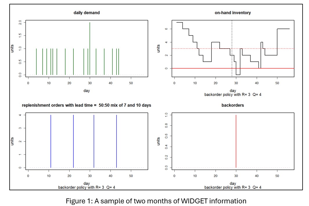
Figure 1 shows two months of WIDGET information. The top left panel shows daily unit demand. The top right shows daily units on hand. The bottom left panel shows the timing and size of replenishment orders back to Acme Products. The bottom right shows units backordered due to stockouts. In this simulation, daily demand was either 0 or 1, with one demand of 2 units. On hand units began the month at 7 and never dropped below 1, though in the next month there was a stockout resulting in a single unit on backorder. Over the two months, there were 4 replenishment orders of 4 units each sent to Acme, all of which arrived during the two-month simulation period.

GOOD TROUBLE DISRUPTS NORMAL OPS

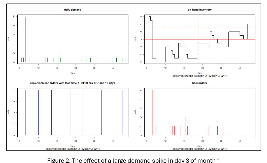
Now we add some “good trouble” to the scenario: An unusually large order arises part way through the planning period. It’s “good” because more demand implies more revenue. But it’s “trouble” because the normal ops inventory control parameters (ROP=3, OQ=4) were not chosen to cope with this situation. The spike in demand might be so big, and so disadvantageously timed, as to overwhelm the inventory system, creating stockouts and their attendant backorders. The KPI report to management for such a month would not be pretty.

Figure 2 shows a scenario in which a demand spike of 10 units hits in the third day of the planning period. In this case, the spike puts the inventory under water for the rest of the month and creates a cascade of backorders extending into the next month. Averaging over 1,000 simulations, month 1 KPI’s show an average on hand of 0.6 units and a miserable 44% fill rate.

FIGHTING BACK WITH IRREGULAR OPERATIONS

Tom’s Spares can respond to an irregular situation with an irregular move by creating an emergency replenishment order. To do it right, they have to think about (a) when to place the order (b) how big the order should be and (c) whether to expedite the order.

The timing question seems obvious: react as soon as the order hits. However, if the customer were to provide early warning, Tom’s Spares could order early and be in better position to limit the disruption from the spike. However, if communication between Tom’s and the customer making the big order is spotty, then the customer might give Tom’s a heads-up later or not at all.

The size of the special order seems obvious too: pre-order the required number of units. But that works best if Tom’s Spares knows when the demand spike will hit. If not, it might be a good idea to order extra to limit the duration of any backorders. In general, the less early warning provided, the larger the order Tom’s should make. This relationship could be explored with simulation, of course.

The arrival of the replenishment order could be left to the usual operation of Acme Products. In the simulations above, Acme was equally likely to respond in 7 or 14 days. For a 28-day planning horizon, taking a risk on getting a 14-day response might be asking for trouble, so it may be especially worthwhile for Tom’s to pay Acme for expedited shipping. Maybe overnight, but possibly something cheaper but still relatively fast.

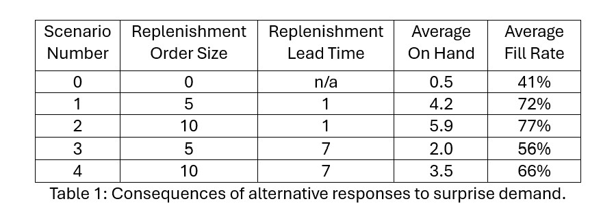
We explored a few more scenarios using simulation. Table 1 shows the results. Scenarios 1-4 assume a surprise additional demand of 10 units arrives on Day 3, triggering an immediate order for  additional replenishment. The size and lead time of the replenishment order varies.

Scenario 0 shows that doing nothing in response to the surprise demand leads to an abysmal 41% fill rate for that month; not shown is that this result sets of the next month for continued poor performance. Regular operations won’t do well. The planner must do something to respond to the anomalous demand.

Doing something in response involves making a one-time emergency replenishment order. The planner must choose the size and timing of that order. Scenarios 1 and 3 depict “half sized” replenishments. Scenarios 1 and 2 depict overnight replenishments, while scenarios 3 and 4 depict guaranteed one week response.

The results make clear that immediate response is more important than the size of the replenishment order for restoring the Fill Rate. Overnight replenishment produces fill rates in the 70% range, while one-week replenishment lead time drops the fill rate into the mid-50% to mid-60% range.

TAKEAWAYS

Inventory management software is expanding from its traditional focus on normal ops to an additional focus on irregular ops (IROPS). This evolution has been made possible by the development of new statistical methods for generating demand scenarios at a daily level.

We considered one IROPS situation: surprise arrival of an anomalously large demand. Daily simulations provided guidance about the timing and size of an emergency replenishment order. Results from such an analysis provide inventory planners with critical backup by estimating the results of alternative interventions that their experience suggests to them.

This video blog holds essential insights for those working with the complexities of inventory management. The session focuses on striking the right balance within the inventory tradeoff curve, inviting viewers to understand the deep-seated importance of this equilibrium. If you’ve ever had to manage stock, you’ll know it feels like a bit of a tug-of-war. On one side, you’re pulling towards less inventory, which is great for saving money but can leave your customers high and dry. On the other, you’re considering more inventory, which keeps your customers happy but can be a pain for your budget. To make a smart choice in this ongoing tug-of-war, you need to understand where your current inventory decisions place you on this tradeoff curve. Are you at a point where you can handle the pressure, or do you need to shuffle along to a more comfortable spot?

If you can’t answer this question, it means that you still rely on outdated methods, risking the potential for surplus inventory or unmet customer needs. Watch the video so you can see exactly where you are on this curve and understand better about whether you want to stay put or move to a more optimal position.

And if you decide to move, we’ve got the tools to guide you. Smart IP&O’s advanced “what-if” analysis enables businesses to precisely evaluate the impact of different inventory strategies, such as adjustments to safety stock levels or changes in reorder points, on their balance between holding costs and service levels. By simulating demand scenarios and inventory policies, Smart IP&O provides a clear visualization of potential financial outcomes and service level implications, allowing for data-driven strategic decisions. This powerful tool ensures businesses can achieve an optimal balance, minimizing excess inventory and related costs while maintaining high service levels to meet customer demand efficiently.  

MRO organizations exist in a wide range of  industries, including public transit, electrical utilities, wastewater, hydro power, aviation, and mining. To get their work done, MRO professionals use Enterprise Asset Management (EAM) and Enterprise Resource Planning (ERP) systems. These systems are designed to do a lot of jobs. Given their features, cost, and extensive implementation requirements, there is an assumption that EAM and ERP systems can do it all.

For example, at a recent Maximo Utilities Working Group event, several prospects stated that “Our EAM will do that” when asked about requirements for forecasting usage, netting out supply plans, and optimizing inventory policies. They were surprised to learn it did not and wanted to know more.

In this post, we summarize the need for add-on software that addresses specialized analytics for inventory optimization, forecasting, and service parts planning.   

EAM Systems

EAM systems can’t ingest forecasts of future usage – these systems simply aren’t designed to conduct supply planning and many don’t even have a place to hold forecasts. So, when an MRO business needs to net out known requirements for planned production or capital projects, an add-on application like Smart IP&O is needed.

Inventory Optimization software with features that support planning known future demand will take project-based data not maintained in the EAM system (including project start dates, duration, and when each part is expected to be needed) and compute a period-by-period forecast over any planning horizon. That “planned” forecast can be projected alongside statistical forecasts of “unplanned” demand arising from normal wear and tear. At that point, parts planning software can net out the supply and identify gaps between supply and demand. This ensures that these gaps won’t go unnoticed and result in shortages that would otherwise delay the completion of the projects. It also minimizes excess stock that would otherwise be ordered too soon and needlessly consumes cash and warehouse space. Again, MRO businesses sometimes mistakenly assume that these capabilities are addressed by their EAM package.

ERP Systems

ERP systems, on the other hand, typically do include an MRP module that is designed to ingest a forecast and net out material requirements. Processing will consider current on hand inventory, open sales orders, scheduled jobs, incoming purchase orders, any bill of materials, and items in transit while transferring between sites. It will compare those current state values to the replenishment policy fields plus any monthly or weekly forecasts to determine when to suggest replenishment (a date) and how much to replenish (a quantity).

So, why not use the ERP system alone to net out the supply plan to prevent shortages and excess? First, while ERP systems have a placeholder for a forecast and some systems can net out supply using their MRP modules, they don’t make it easy to reconcile planned demand requirements associated with capital projects. Most of the time, the data on when planned projects will occur is maintained outside of the ERP, especially the project’s bill of materials detailing what parts will be needed to support the project. Second, many ERP systems don’t offer anything effective when it comes to predictive capabilities, relying instead on simple math that just won’t work for service parts due to the high prevalence of intermittent demand. Finally, ERP systems don’t have flexible user-friendly interfaces that support interacting with the forecasts and supply plan.

Reorder Point Logic

Both ERP and EAM have placeholders for reorder point replenishment methods such as Min/Max levels. You can use inventory optimization software to populate these fields with the risk-adjusted reorder point policies. Then within the ERP or EAM systems, orders are triggered whenever actual (not forecasted) demand drives on-hand stock below the Min. This type of policy doesn’t use a traditional forecast that projects demand week-over-week or month-over-month and is often referred to as “demand driven replenishment” (since orders only occur when actual demand drives stock below a user defined threshold).

But just because it isn’t using a period-over-period forecast doesn’t mean it isn’t being predictive. Reorder point policies should be based on a prediction of demand over a replenishment lead time plus a buffer to protect against demand and supply variability. MRO businesses need to know the stockout risk they are incurring with any given stocking policy. After all, inventory management is risk management – especially in MRO businesses when the cost of stockout is so high. Yet, ERP and EAM do not offer any capabilities to risk-adjust stocking policies. They force users to manually generate these policies externally or to use basic rule of thumb math that doesn’t detail the risks associated with the choice of policy.

Summary

Supply chain planning functionality such as inventory optimization isn’t the core focus of EAM  and ERP. You should leverage add-on planning platforms, like Smart IP&O, that support statistical forecasting, planned project management, and inventory optimization. Smart IP&O will develop forecasts and stocking policies that can be input to an EAM or ERP system to drive daily ordering.

Our customers have usually settled into one way to manage their service parts inventory. The professor in me would like to think that the chosen inventory policy was a reasoned choice among considered alternatives, but more likely it just sort of happened. Maybe the inventory honcho from long ago had a favorite and that choice stuck. Maybe somebody used an EAM or ERP system that offered only one choice. Perhaps there were some guesses made, based on the conditions at the time.

The Competitors

Too seldom, businesses make these choices in haphazard ways. But modern service parts planning software lets you be more systematic about your choices. This post demonstrates that proposition by making objective comparisons among three popular inventory policies:  Order Up To, Reorder Point/Order Quantity, and Min/Max.  I discussed each of these policies in this video blog.

• Order Up To. This is a periodic review policy where every T days, on-hand inventory is tallied and an order of random size is placed to bring the stock level back up to S units.
• Q, R or Reorder Point/Order Quantity. Q, R is a continuous review policy where every day, inventory is tallied. If there are Q or fewer units on hand, an order of fixed size is placed for R more units.
• Min, Max is another continuous review policy where every day, inventory is tallied. If there are Min or fewer units on hand, an order is placed to bring the stock level back up to Max units.

Inventory theory says these choices are listed in increasing order of effectiveness. The first option, Order Up To, is clearly the simplest and cheapest to implement, but it closes its eyes to what’s going on for long periods of time.  Imposing a specified passage of time in between orders makes it, in theory, less flexible. In contrast, the two continuous review options keep an eye on what’s happening all the time, so they can react to potential stockouts quicker. The Min/Max option is, in theory, more flexible than the option that uses a fixed reorder quantity because the size of the order dynamically changes to accommodate the demand.

That’s the theory. This post examines evidence from head-to-head comparisons to check the theory and put concrete numbers on the relative performance of the three policies.

The Meaning of “Best”

How should we keep score in this tournament? If you are a regular reader of this Smart Forecaster blog, you know that the core of inventory planning is a tug-of-war between two opposing objectives: keeping inventory lean vs keeping item availability metrics such as service level high.

To simplify things, we will compute “one number to rule them all”: the average operating cost. The winning policy will be the one with the lowest average.

This average is the sum of three components: the cost of holding inventory (“holding cost”), the cost of ordering replenishment units (“ordering cost”) and the cost of losing a sale (“shortage cost”). To make things concrete, we used the following assumptions:

• Each service part is valued at $1,000.
• Annual holding cost is 10% of item value, or $100 per year per unit.
• Processing each replenishment order costs $20 per order.
• Each unit demanded but not provided costs the value of the part, $1,000.

For simplicity, we will refer to the average operating cost as simply “the cost”.

Of course, the lowest average cost can be achieved by getting out of the business. So the competition required a performance constraint on item availability: Each option had to achieve a fill rate of at least 99%.

The Alternatives Duke it Out

A key element of context is whether stockouts result in losses or backorders. Assuming that the service part in question is critical, we assumed that unfilled orders are lost, which means that a competitor fills the order. In an MRO environment, this will mean additional downtime due to stockout.

To compare the alternatives, we used our predictive modeling engine to run a large number of Monte Carlo simulations.  Each simulation involved specifying the parameter values of each policy (e.g., Min and Max values), generating a demand scenario, feeding that into the logic of the policy, and measuring the resulting cost averaged over 365 days of operation. Repeating this process 1,000 times and averaging the 1,000 resulting costs gave the final result for each policy.  

To make the comparison fair, each alternative had to be designed for its best performance. So we searched the “design space” of each policy to find the design with the lowest cost. This required repeating the process described in the previous paragraph for many pairs of parameter values and identifying the pair yielding the lost average annual operating cost.

Using the algorithms in Smart Inventory Optimization (SIO^TM) we made head-to-head-to-head comparisons under the following assumptions about demand and supply:

• Item demand was assumed to be intermittent and highly variable but relatively simple in that there was neither trend nor seasonality, as is often true for service parts. Daily mean demand was 5 units with a large standard deviation of 13 units. Figure 1 shows a sample of one year’s demand. We have chosen a very challenging demand pattern, in which some days have 10 to even 20 times the average demand.

Figure 1: Daily part demand was assumed to be intermittent and very spikey.

​​

• Suppliers’ replenishment lead times were 14 days 75% of the time and 21 days otherwise. This reflects the fact that there is always uncertainty in the supply chain.

And the Winner Is…

Was the theory right? Kinda’ sorta’.

Table 1 shows the results of the simulation experiments. For each of the three competing policies, it shows the average annual operating cost, the margin of error (technically, an approximate 95% confidence interval for the mean cost), and the apparent best choices for parameter values.

Table 1: Results of the simulated comparisons

For example, the average cost for the (T,S) policy when T is fixed at 30 days was $41,680. But the Plus/Minus implies that the results are compatible with a “true” cost (i.e., the estimate from an infinite number of simulations) of anywhere between $39,890 and $43,650. The reason there is so much statistical uncertainty is the extremely spikey nature of demand in this example.

Table 1 says that, in this example, the three policies fall in line with expectations. However, more useful conclusions would be:

1. The three policies are remarkably similar in average cost. By clever choice of parameter values, one can get good results out of any of the three policies.
2. Not shown in Table 1, but clear from the detailed simulation results, is that poor choices for parameter values can be disastrous for any policy.
3. It is worth noting that the periodic review (T,S) policy was not allowed to optimize over possible values of T. We fixed T at 30 to mimic what is common in practice, but those who use the periodic review policy should consider other review periods. An additional experiment fixed the review period at T = 7 days. The average cost in this scenario was minimized at $36,551 ± $1,668 with S = 343. This result is better than that using T = 30 days.
4. We should be careful about over-generalizing these results. They depend on the assumed values of the three cost parameters (holding, ordering and shortage) and the character of the demand process.
5. It is possible to run experiments like those shown here automatically in Smart Inventory Optimization. This means that you too would be able to explore design choices in a rigorous way.

​In a highly configurable manufacturing environment, forecasting finished goods can become a complex and daunting task. The number of possible finished products will skyrocket when many components are interchangeable. A traditional MRP would force us to forecast every single finished product which can be unrealistic or even impossible. Several leading ERP solutions introduce the concept of the “Planning BOM”, which allows the use of forecasts at a higher level in the manufacturing process. In this article, we will discuss this functionality in ERP, and how you can take advantage of it with Smart Inventory Planning and Optimization (Smart IP&O) to get ahead of your demand in the face of this complexity.

Why Would I Need a Planning BOM?

Traditionally, each finished product or SKU would have a rigidly defined bill of materials. If we stock that product and want to plan around forecasted demand, we would forecast demand for those products and then feed MRP to blow this forecasted demand from the finished good level down to its components via the BOM.

Many companies, however, offer highly configurable products where customers can select options on the product they are buying. As an example, recall the last time you bought a personal computer. You chose a brand and model, but from there, you were likely presented with options: what speed of CPU do you want? How much RAM do you want? What kind of hard drive and how much space? If that business wants to have these computers ready and available to ship to you in a reasonable time, suddenly they are no longer just anticipating demand for that model—they must forecast that model for every type of CPU, for all quantities of RAM, for all types of hard drive, and all possible combinations of those as well! For some manufacturers, these configurations can compound to hundreds or thousands of possible finished good permutations.

There may be so many possible customizations that the demand at the finished product level is completely unforecastable in a traditional sense. Thousands of those computers may sell every year, but for each possible configuration, the demand may be extremely low and sporadic—perhaps certain combinations sell once and never again.

This often forces these companies to plan reorder points and safety stock levels mostly at the component level, while largely reacting to firm demand at the finished good level via MRP. While this is a valid approach, it lacks a systematic way to leverage forecasts that may account for anticipated future activity such as promotions, upcoming projects, or sales opportunities. Forecasting at the “configured” level is effectively impossible, and trying to weave in these forecast assumptions at the component level isn’t feasible either.

Planning BOM Explained

This is where Planning BOMs come in. Perhaps the sales team is working a big b2b opportunity for that model, or there’s a planned promotion for Cyber Monday. While trying to work in those assumptions for every possible configuration isn’t realistic, doing it at the model level is totally doable—and tremendously valuable.

The Planning BOM can use a forecast at a higher level and then blow demand down based on predefined proportions for its possible components. For example, the computer manufacturer may know that most people opt for 16GB of RAM, and far fewer opt for the upgrades to 32 or 64. The planning BOM allows the organization to (for example) blow 60% of the demand down to the 16GB option, 30% to the 32GB option, and 10% to the 64GB option. They could do the same for CPUs, hard drives, or any other customizations available.  

The business can now focus their forecast at this model level, leaving the Planning BOM to figure out the component mix. Clearly, defining these proportions requires some thought, but Planning BOMs effectively allow businesses to forecast what would otherwise be unforecastable.

The Importance of a Good Forecast

Of course, we still need a good forecast to load into an ERP system. As explained in this article, while ERP  can import a forecast, it often cannot generate one and when it does it tends to require a great deal of hard to use configurations that don’t often get revisited resulting in inaccurate forecasts.  It is therefore up to the business to come up with their own sets of forecasts, often manually produced in Excel. Forecasting manually generally presents a number of challenges, including but not limited to:

• The inability to identify demand patterns like seasonality or trend
• Overreliance on customer or sales forecasts
• Lack of accuracy or performance tracking

No matter how well configured the MRP is with your carefully considered Planning BOMs, a poor forecast means poor MRP output and mistrust in the system—garbage in, garbage out. Continuing along with the “computer company” example, without a systematic way of capturing key demand patterns and/or domain knowledge in the forecast, MRP can never see it.

Extend ERP  with Smart IP&O

Smart IP&O is designed to extend your ERP system with a number of integrated demand planning and inventory optimization solutions. For example, it can generate statistical forecasts automatically for large numbers of items, allows for intuitive forecast adjustments, tracks forecast accuracy, and ultimately allows you to generate true consensus-based forecasts to better anticipate the needs of your customers.

Thanks to highly flexible product hierarchies, Smart IP&O is perfectly suited to forecasting at the Planning BOM level so you can capture key patterns and incorporate business knowledge at the levels that matter most. Furthermore you can analyze and deploy optimal safety stock levels at any level of your BOM.

For too many companies, a critical piece of data fact-finding ― the measurement of demand uncertainty ― is handled by simple but inaccurate rules of thumb.  For example, demand planners will often compute safety stock by a user-defined multiple of the forecast or historical average.  Or they may configure their ERP to order more when on hand inventory gets to 2 x the average demand over the lead time for important items and 1.5 x for less important ones. This is a huge mistake with costly consequences.

The choice of multiple ends up being a guessing game.  This is because no human being can compute exactly how much inventory to stock considering all the uncertainties.  Multiples of the average lead time demand are simple to use but you can never know whether the multiple used is too large or too small until it is too late.  And once you know, all the information has changed, so you must guess again and then wait and see how the latest guess turns out.  With each new day, you have new demand, new details on lead times, and the costs may have changed.  Yesterday’s guess, no more matter how educated is no longer relevant today.  Proper inventory planning should be void of inventory and forecast guesswork.  Decisions must be made with incomplete information but guessing is not the way to go.

Knowing how much to buffer requires a fact-based statistical analysis that can accurately answer questions such as:

• How much extra stock is needed to improve service levels by 5%
• What the hit to on-time delivery will be if inventory is reduced by 5%
• What service level target is most profitable.
• How will the stockout risk be impacted by the random lead times we face.

Intuition can’t answer these questions, doesn’t scale across thousands of parts, and is often wrong.  Data, probability math and modern software are much more effective. Winging it is not the path to sustained excellence.