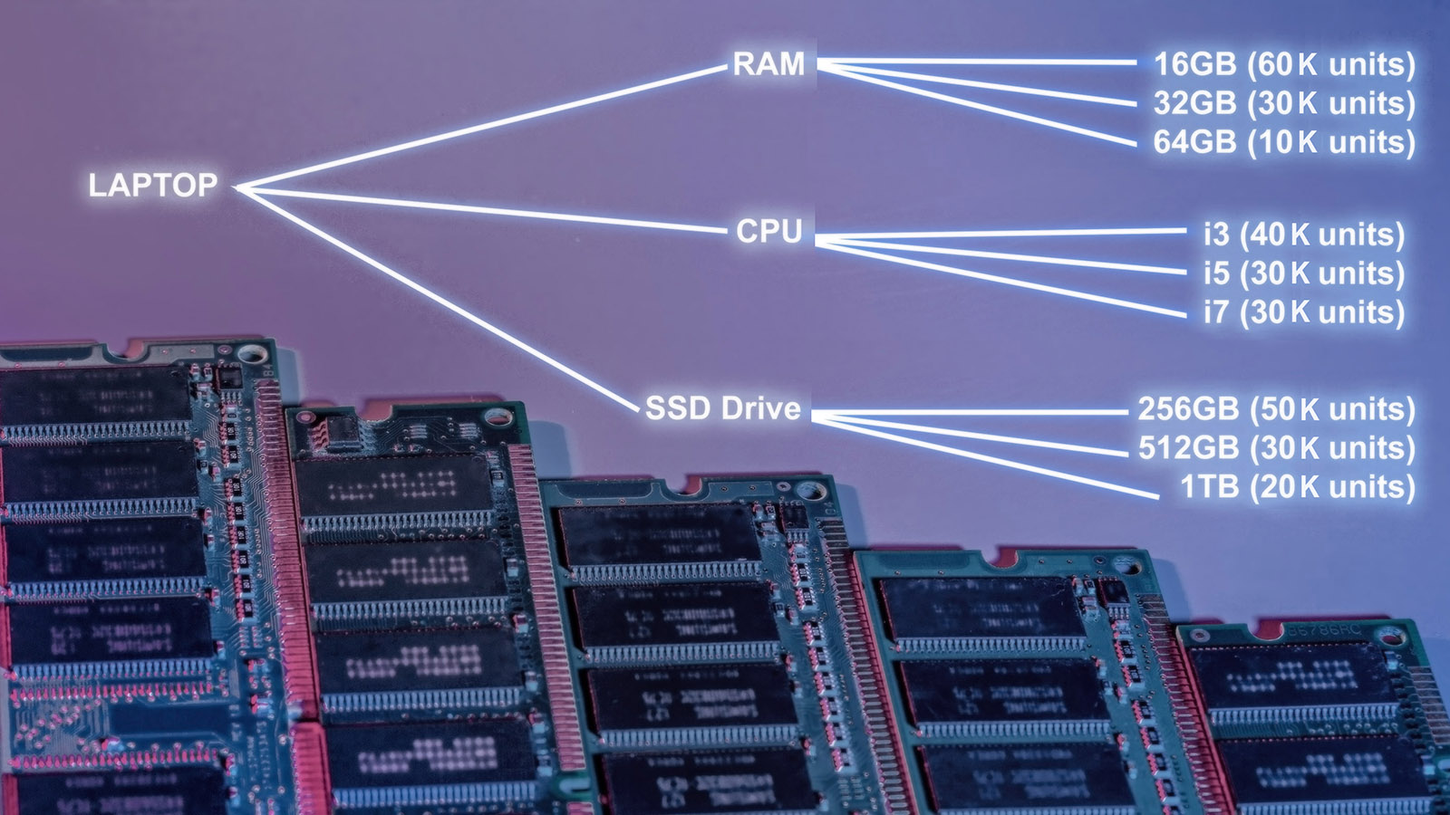
The Cost of Spreadsheet Planning

Companies that depend on spreadsheets for demand planning, forecasting, and inventory management are often constrained by the spreadsheet’s inherent limitations. This post examines the drawbacks of traditional inventory management approaches caused by spreadsheets and their associated costs, contrasting these with the significant benefits gained from embracing state-of-the-art planning technologies.

Spreadsheets, while flexible for their infinite customizability, are fundamentally manual in nature requiring significant data management, human input, and oversight. This increases the risk of errors, from simple data entry mistakes to complex formula errors, that cause cascading effects that adversely impact forecasts.  Additionally, despite advances in collaborative features that enable multiple users to interact with a common sheet, spreadsheet-based processes are often siloed. The holder of the spreadsheet holds the data.  When this happens, many sources of data truth begin to emerge.  Without the trust of an agreed-upon, pristine, and automatically updated source of data, organizations don’t have the necessary foundation from which predictive modeling, forecasting, and analytics can be built.

In contrast, advanced planning systems like Smart IP&O are designed to overcome these limitations. Such systems are built to automatically ingest data via API or files from ERP and EAM systems, transform that data using built in ETL tools, and can process large volumes of data efficiently.  This enables businesses to manage complex inventory and forecasting tasks with greater accuracy and less manual effort because the data collection, aggregation, and transformation is already done. Transitioning to advanced planning systems is key for optimizing resources for several reasons.

Spreadsheets also have a scaling problem. The bigger the business grows, the greater the number of spreadsheets, workbooks, and formulas becomes.  The result is a tightly wound and rigid set of interdependencies that become unwieldy and inefficient.  Users will struggle to handle the increased load and complexity with slow processing times and an inability to manage large datasets and face challenges collaborating across teams and departments.

On the other hand, advanced planning systems for inventory optimization, demand planning, and inventory management are scalable, designed to grow with the business and adapt to its changing needs. This scalability ensures that companies can continue to manage their inventory and forecasting effectively, regardless of the size or complexity of their operations. By transitioning to systems like Smart IP&O, companies can not only improve the accuracy of their inventory management and forecasting but also gain a competitive edge in the market by being more responsive to changes in demand and more efficient in their operations.

Benefits of Jumping in: An electric utility company struggled to maintain service parts availability without overstocking for over 250,000-part numbers across a diverse network of power generation and distribution facilities. It replaced their twenty-year-old legacy planning process that made heavy use of spreadsheets with Smart IP&O and a real-time integration to their EAM system.  Before Smart, they were only able to modify Min/Max and Safety Stock levels infrequently.  When they did, it was nearly always because a problem occurred that triggered the review.  The methods used to change the stocking parameters relied heavily on gut feel and averages of the historical usage.   The Utility leveraged Smart’s what-if scenarios to create digital twins of alternate stocking policies and simulated how each scenario would perform across key performance indicators such as inventory value, service levels, fill rates, and shortage costs.  The software pinpointed targeted Min/Max increases and decreases that were deployed to their EAM system, driving optimal replenishments of their spare parts.  The result:  A significant inventory reduction of $9 million that freed up cash and valuable warehouse space while sustaining 99%+ target service levels.

Managing Forecast Accuracy: Forecast error is an inevitable part of inventory management, but most businesses don’t track it.  As Peter Drucker said, “You can’t improve what you don’t measure.”  A global high-tech manufacturing company utilizing a spreadsheet-based forecast process had to manually create its baseline forecasts and forecast accuracy reporting.  Given the planners’ workload and siloed processes, they just didn’t update their reports very often, and when they did, the results had to be manually distributed.  The business didn’t have a way of knowing just how accurate a given forecast was and couldn’t cite their actual errors by group of part with any confidence.  They also didn’t know whether their forecasts were outperforming a control method.  After Smart IP&O went live, the Demand Planning module automated this for them. Smart Demand Planner now automatically reforecasts their demand each planning cycle utilizing ML methods and saves accuracy reports for every part x location.  Any overrides that are applied to the forecasts can now be auto-compared to the baseline to measure forecast value add – i.e., whether the additional effort to make those changes improved the accuracy.  Now that the ability to automate the baseline statistical forecasting and produce accuracy reports is in place, this business has solid footing from which to improve their forecast process and resulting forecast accuracy.

Get it Right and Keep it Right:  Another customer in the aftermarket parts business has used Smart’s forecasting solutions since 2005 – nearly 20 years!  They were faced with challenges forecasting intermittently demanded parts sold to support their auto aftermarket business. By replacing their spreadsheet-based approach and manual uploads to SAP with statistical forecasts of demand and safety stock from SmartForecasts, they were able to significantly reduce backorders and lost sales, with fill rates improving from 93% to 96% within just three months.  The key to their success was leveraging Smart’s patented method for forecasting intermittent demand – The “Smart-Willemain” bootstrap method generated accurate estimates of the cumulative demand over the lead time that helped ensure better visibility of the possible demands.

Connecting Forecasts to the Inventory Plan: Advanced planning systems support forecast-based inventory management, which is a proactive approach that relies on demand forecasts and simulations to predict possible outcomes and their associated probabilities.  This data is used to determine optimal inventory levels.  Scenario-based or probabilistic forecasting contrasts with the more reactive nature of spreadsheet-based methods. A longtime customer in the fabric business, previously dealt with overstocks and stockouts due to intermittent demand for thousands of SKUs. They had no way of knowing what their stock-out risks were and so couldn’t proactively modify policies to mitigate risk other than making very rough-cut assumptions that tended to overstock grossly.  They adopted Smart Software’s demand and inventory planning software to generate simulations of demand that identified optimal Minimum On-Hand values and order quantities, maintaining product availability for immediate shipping, highlighting the advantages of a forecast-based inventory management approach.

Better Collaboration:  Sharing forecasts with key suppliers helps to ensure supply.  Kratos Space, part of Kratos Defense & Security Solutions, Inc., leveraged Smart forecasts to provide their Contract Manufacturers with better insights on future demand.  They used the forecasts to make commitments on future buys that enabled the CM to reduce material costs and lead times for engineered-to-order systems. This collaboration demonstrates how advanced forecasting techniques can lead to significant supply chain collaboration that yields efficiencies and cost savings for both parties.


Weathering a Demand Forecast

For some of our customers, weather has a significant influence on demand. Extreme short-term weather events like fires, droughts, hot spells, and so forth can have a significant near-term influence on demand.

There are two ways to factor weather into a demand forecast: indirectly and directly. The indirect route is easier using the scenario-based approach of Smart Demand Planner. The direct approach requires a tailored special project requiring additional data and hand-crafted modeling.

Indirect Accounting for Weather

The standard model built into Smart Demand Planner (SDP) accommodates weather effects in four ways:

  1. If the world is steadily getting warmer/colder/drier/wetter in ways that impact your sales, SDP detects these trends automatically and incorporates them into the demand scenarios it generates.
  2. If your business has a regular rhythm in which certain days of the week or certain months of the year have consistently higher or lower-than-average demand, SDP also automatically detects this seasonality and incorporates it into its demand scenarios.
  3. Often it is the cussed randomness of weather that interferes with forecast accuracy. We often refer to this effect as “noise”. Noise is a catch-all term that incorporates all kinds of random trouble. Besides weather, a geopolitical flareup, the surprise failure of a regional bank, or a ship getting stuck in the Suez Canal can and have added surprises to product demand. SDP assesses the volatility of demand and reproduces it in its demand scenarios.
  4. Management overrides. Most of the time, customers let SDP churn away to automatically generate tens of thousands of demand scenarios. But if users feel the need to touch up specific forecasts using their insider knowledge, SDP can make that happen through management overrides.

Direct Accounting for Weather

Sometimes a user will be able to articulate subject matter expertise linking factors outside their company (such as interest rates or raw materials costs or technology trends) to their own aggregate sales. In these situations, Smart Software can arrange for one-off special projects that provide alternative (“causal”) models to supplement our standard statistical forecasting models. Contact your Smart Software representative to discuss a possible causal modeling project.

Meanwhile, don’t forget your umbrella.


Leveraging ERP Planning BOMs with Smart IP&O to Forecast the Unforecastable

​In a highly configurable manufacturing environment, forecasting finished goods can become a complex and daunting task. The number of possible finished products will skyrocket when many components are interchangeable. A traditional MRP would force us to forecast every single finished product which can be unrealistic or even impossible. Several leading ERP solutions introduce the concept of the “Planning BOM”, which allows the use of forecasts at a higher level in the manufacturing process. In this article, we will discuss this functionality in ERP, and how you can take advantage of it with Smart Inventory Planning and Optimization (Smart IP&O) to get ahead of your demand in the face of this complexity.

Why Would I Need a Planning BOM?

Traditionally, each finished product or SKU would have a rigidly defined bill of materials. If we stock that product and want to plan around forecasted demand, we would forecast demand for those products and then feed MRP to blow this forecasted demand from the finished good level down to its components via the BOM.

Many companies, however, offer highly configurable products where customers can select options on the product they are buying. As an example, recall the last time you bought a personal computer. You chose a brand and model, but from there, you were likely presented with options: what speed of CPU do you want? How much RAM do you want? What kind of hard drive and how much space? If that business wants to have these computers ready and available to ship to you in a reasonable time, suddenly they are no longer just anticipating demand for that model—they must forecast that model for every type of CPU, for all quantities of RAM, for all types of hard drive, and all possible combinations of those as well! For some manufacturers, these configurations can compound to hundreds or thousands of possible finished good permutations.

Planning BOM emphasizing the large numbers of permutations Laptops Factory Components

There may be so many possible customizations that the demand at the finished product level is completely unforecastable in a traditional sense. Thousands of those computers may sell every year, but for each possible configuration, the demand may be extremely low and sporadic—perhaps certain combinations sell once and never again.

This often forces these companies to plan reorder points and safety stock levels mostly at the component level, while largely reacting to firm demand at the finished good level via MRP. While this is a valid approach, it lacks a systematic way to leverage forecasts that may account for anticipated future activity such as promotions, upcoming projects, or sales opportunities. Forecasting at the “configured” level is effectively impossible, and trying to weave in these forecast assumptions at the component level isn’t feasible either.


Planning BOM Explained

This is where Planning BOMs come in. Perhaps the sales team is working a big b2b opportunity for that model, or there’s a planned promotion for Cyber Monday. While trying to work in those assumptions for every possible configuration isn’t realistic, doing it at the model level is totally doable—and tremendously valuable.

The Planning BOM can use a forecast at a higher level and then blow demand down based on predefined proportions for its possible components. For example, the computer manufacturer may know that most people opt for 16GB of RAM, and far fewer opt for the upgrades to 32 or 64. The planning BOM allows the organization to (for example) blow 60% of the demand down to the 16GB option, 30% to the 32GB option, and 10% to the 64GB option. They could do the same for CPUs, hard drives, or any other customizations available.  

Planning BOM Explained with computer random access memory ram close hd


The business can now focus their forecast at this model level, leaving the Planning BOM to figure out the component mix. Clearly, defining these proportions requires some thought, but Planning BOMs effectively allow businesses to forecast what would otherwise be unforecastable.


The Importance of a Good Forecast

Of course, we still need a good forecast to load into an ERP system. As explained in this article, while ERP  can import a forecast, it often cannot generate one and when it does it tends to require a great deal of hard to use configurations that don’t often get revisited resulting in inaccurate forecasts.  It is therefore up to the business to come up with their own sets of forecasts, often manually produced in Excel. Forecasting manually generally presents a number of challenges, including but not limited to:

  • The inability to identify demand patterns like seasonality or trend
  • Overreliance on customer or sales forecasts
  • Lack of accuracy or performance tracking

No matter how well configured the MRP is with your carefully considered Planning BOMs, a poor forecast means poor MRP output and mistrust in the system—garbage in, garbage out. Continuing along with the “computer company” example, without a systematic way of capturing key demand patterns and/or domain knowledge in the forecast, MRP can never see it.


Extend ERP  with Smart IP&O

Smart IP&O is designed to extend your ERP system with a number of integrated demand planning and inventory optimization solutions. For example, it can generate statistical forecasts automatically for large numbers of items, allows for intuitive forecast adjustments, tracks forecast accuracy, and ultimately allows you to generate true consensus-based forecasts to better anticipate the needs of your customers.

Thanks to highly flexible product hierarchies, Smart IP&O is perfectly suited to forecasting at the Planning BOM level so you can capture key patterns and incorporate business knowledge at the levels that matter most. Furthermore you can analyze and deploy optimal safety stock levels at any level of your BOM.


You Need to Team up with the Algorithms

Over forty years ago, Smart Software consisted of three friends working to start a company in a church basement. Today, our team has expanded to operate from multiple locations across Massachusetts, New Hampshire and Texas, with team members in England, Spain, Armenia and India. Like many of you in your jobs,  we have found ways to make distributed teams work for us and for you.

This note is about a different kind of teamwork: the collaboration between you and our software that happens at your fingertips. I often write about the software itself and what goes on “under the hood”. This time, my subject is how you should best team up with the software.

Our software suite, Smart Inventory Planning and Optimization (Smart IP&O™) is capable of massively detailed calculations of future demand and the inventory control parameters (e.g., reorder points and order quantities) that would most effectively manage that demand. But your input is required to make the most of all that power. You need to team up with the algorithms.

That interaction can take several forms. You can start by simply assessing how you are doing now. The report writing functions in Smart IP&O (Smart Operational Analytics™) can collate and analyze all your transactional data to measure your Key Performance Indicators (KPIs), both financial (e.g., inventory investment) and operational (e.g., fill rates).

The next step might be to use SIO (Smart Inventory Optimization™), the inventory analytics within SIP&O, to play “what-if” games with the software. For example, you might ask “What if we reduced the order quantity on item 1234 from 50 to 40?” The software grinds the numbers to let you know how that would play out, then you react. This can be useful, but what if you have 50,000 items to consider? You would want to do what-if games for a few critical items, but not all of them.

The real power comes with using the automatic optimization capability in SIO. Here you can team with the algorithms at scale. Using your business judgement, you can create “groups”, i.e., collections of items that share some critical features. For example, you might create a group for “critical spare parts for electric utility customers” consisting of 1,200 parts. Then again calling on your business judgement, you could specify what item availability standard should apply to all the items in that group (e.g., “at least 95% chance of not stocking out in a year”). Now the software can take over and automatically work out the best reorder points and order quantities for every one of those items to achieve your required item availability at the lowest possible total cost. And that, dear reader, is powerful teamwork.


A Rough Map of Forecasting-Related Terms

People new to the jobs of “demand planner” or “supply planner” are likely to have questions about the various forecasting terms and methods used in their jobs. This note may help by explaining these terms and showing how they relate.


Demand Planning

Demand planning is about how much of what you have to sell will go out the door in the future, e.g., how many what-nots you will sell next quarter. Here are six methodologies often used in demand planning.

  • Statistical Forecasting
    • These methods use demand history to forecast future values. The two most common methods are curve fitting and data smoothing.
    • Curve fitting matches a simple mathematical function, like the equation for a straight line (y= a +b∙t) or an interest-rate type curve (y=a∙bt), to the demand history. Then it extends that line or curve forward in time as the forecast.
    • In contrast, data smoothing does not result in an equation. Instead it sweeps through the demand history, averaging values along the way, to create a smoother version of the history. These methods are called exponential smoothing and moving average. In the simplest case (i.e., in the absence of trend or seasonality, for which variants exist), the goal is to estimate the current average level of demand and use that as the forecast.
    • These methods produce “point forecasts”, which are single-number estimates for each future time period (e.g., “Sales in March will be 218 units”). Sometimes they come with estimates of potential forecast error bolted on using separate models of demand variability (“Sales in March will be 218 ± 120 units”).
  • Probabilistic Forecasting
    • This approach keys on the randomness of demand and works hard to estimate forecast uncertainty. It regards forecasting less as an exercise in cranking out specific numbers and more as an exercise in risk management.
    • It explicitly models the variability in demand and uses that to present results in the form of large numbers of scenarios constructed to show the full range of possible demand sequences. These are especially useful in tactical supply planning tasks, such as setting reorder points and order quantities.
  • Causal Forecasting
    • Statistical forecasting models use as inputs only the past demand history of the item in question. They regard the up-and-down wiggles in the demand plot as the end result of myriad unnamed factors (interest rates, the price of tea in China, phases of the moon, whatever). Causal forecasting explicitly identifies one or more influences (interest rates, advertising spend, competitors’ prices, …) that could plausibly influence sales. Then it builds an equation relating the numerical values of these “drivers” or “causal factors” to item sales. The equation’s coefficients are estimated by “regression analysis”.
  • Judgemental Forecasting
    • Golden Gut. Despite the general availability of gobs of data, some companies pay little attention to the numbers and give greater weight to the subjective judgements of an executive deemed to have a “Golden Gut”, which allows him or her to use “gut feel” to predict what future demand will be. If that person has great experience, has spent a career actually looking at the numbers, and is not prone to wishful thinking or other forms of cognitive bias, the Golden Gut can be a cheap, fast way to plan. But there is good evidence from studies of companies run this way that relying on the Golden Gut is risky.
    • Group Consensus. More common is a process that uses a periodic meeting to create a group consensus forecast. The group will have access to shared objective data and forecasts, but members will also have knowledge of factors that may not be measured well or at all, such as consumer sentiment or the stories relayed by sales reps. It is helpful to have a shared, objective starting point for these discussions consisting of some sort of objective statistical analysis. Then the group can consider adjusting the statistical forecast. This process anchors the forecast in objective reality but exploits all the other information available outside the forecasting database.
    • Scenario Generation. Sometimes several people will meet and discuss “strategic what-if” questions. “What if we lose our Australian customers?” “What if our new product roll-out is delayed by six months?” “What if our sales manager for the mid-west jumps to a competitor?” These bigger-picture questions can have implications for item-specific forecasts and might be added to any group-consensus forecasting meeting.
  • New product forecasting
    • New products, by definition, have no sales history to support statistical, probability, or causal forecasting. Subjective forecasting methods can always be used here, but these often rely on a dangerous ratio of hopes to facts. Fortunately, there is at least partial support for objective forecasting in the form of curve fitting.
    • A graph of the cumulative sales of an item often describes some sort of “S-curve”, i.e., a graph that starts at zero, builds up, then levels off to a final lifetime total sales. The curve gets its name because it looks like a letter S somehow smeared and stretched to the right. Now there are an infinite number of S-curves, so forecasters typically pick an equation and subjectively specify some key parameter values, like when sales will hit 25%, 50% and 75% of total lifetime sales and what that final level will be. This is also overtly subjective, but it produces detailed period-by-period forecasts that can be updated as experience builds up. Finally, S-curves are sometimes shaped to match the known history of a similar, predecessor product (“Sales for our last gizmo looked like this, so let’s use that as a template.”).


Supply Planning

Demand planning feeds into supply planning by predicting future sales (e.g., for finished goods) or usage (e.g., for spare parts). Then it is up to supply planning to make sure the items in question will be available to sell or to use.

  • Dependent demand
    • Dependent demand is demand that can be determined by its relationship to demand for another item. For instance, a bill of materials may show that a little red wagon consists of a body, a pull bar, four wheels, two axles, and various fasteners to keep the wheels on the axles and connect the pull bar to the body. So if you hope to sell 10 little red wagons, you’d better make 10, which means you need 10×2 = 20 axles, 10×4 = 40 wheels, etc. Dependent demand governs raw materials purchasing, component and subsystems purchasing, even personnel hiring (10 wagons need one high-school kid to put them together over a 1 hour shift).
    • If you have multiple products with partially overlapping bills of materials, you have a choice of two forecasting approaches. Suppose you sell not only little red wagons but little blue baby carriages and that both use the same axles. To predict the number of axles you need you could (1) predict the dependent demand for axles from each product and add the forecasts or (2) observe the total demand history for axles as its own time series and forecast that separately. Which works better is an empirical question that can be tested.
  • Inventory management
    • Inventory management entails many different tasks. These include setting inventory control parameters such as reorder points and order quantities, reacting to contingencies such as stockouts and order expediting, setting staffing levels, and selecting suppliers.
  • Forecasting plays a role in the first three. The number of replenishment orders that will be made in a year for each product determines how many people are needed to cut PO’s. The number and severity of stockouts in a year determines the number of contingencies that must be handled. The number of PO’s and stockouts in a year will be random but be governed by the choices of inventory control parameters. The implications of any such choices can be modeled by inventory simulations. These simulations will be driven by detailed demand scenarios generated by probabilistic forecasts.


Six Demand Planning Best Practices You Should Think Twice About

Every field, including forecasting, accumulates folk wisdom that eventually starts masquerading as “best practices.”  These best practices are often wise, at least in part, but they often lack context and may not be appropriate for certain customers, industries, or business situations.  There is often a catch, a “Yes, but”. This note is about six usually true forecasting precepts that nevertheless do have their caveats.


  1. Organize your company around a one-number forecast. This sounds sensible: it’s good to have a shared vision. But each part of the company will have its own idea about which number is the number. Finance may want quarterly revenue, Marketing may want web site visits, Sales may want churn, Maintenance may want mean time to failure. For that matter, each unit probably has a handful of key metrics. You don’t need a slogan – you need to get your job done.


  1. Incorporate business knowledge into a collaborative forecasting process. This is a good general rule, but if your collaborative process is flawed, messing with a statistical forecast via management overrides can decrease accuracy. You don’t need a slogan – you need to measure and compare the accuracy of any and all methods and go with the winners.


  1. Forecast using causal modeling. Extrapolative forecasting methods take no account of the underlying forces driving your sales, they just work with the results. Causal modeling takes you deeper into the fundamental drivers and can improve both accuracy and insight. However, causal models (implemented through regression analysis) can be less accurate, especially when they require forecasts of the drivers (“predictions of the predictors”) rather than simply plugging in recorded values of lagged predictor variables. You don’t need a slogan: You need a head-to-head comparison.


  1. Forecast demand instead of shipments. Demand is what you really want, but “composing a demand signal” can be tricky: what do you do with internal transfers? One-off’s?  Lost sales? Furthermore, demand data can be manipulated.  For example, if customers intentionally don’t place orders or try to game their orders by ordering too far in advance, then order history won’t be better than shipment history.  At least with shipment history, it’s accurate:  You know what you shipped. Forecasts of shipments are not forecasts of  “demand”, but they are a solid starting point.


  1. Use Machine Learning methods. First, “Machine learning” is an elastic concept that includes an ever-growing set of alternatives. Under the hood of many ML advertised models is just an auto-pick an extrapolative forecast method (i.e., best fit) which while great at forecasting normal demand, has been around since the 1980’s (Smart Software was the first company to release an auto-pick method for the PC).   ML models are data hogs that require larger data sets than you may have available. Properly choosing then training an ML model requires a level of statistical expertise that is uncommon in many manufacturing and distribution businesses. You might want to find somebody to hold your hand before you start playing this game.


  1. Removing outliers creates better forecasts. While it is true that very unusual spikes or drops in demand will mask underlying demand patterns such as trend or seasonality, it isn’t always true that you should remove the spikes. Often these demand surges reflect the uncertainty that can randomly interfere with your business and thus need to be accounted for.  Removing this type of data from your demand forecast model might make the data more predictable on paper but will leave you surprised when it happens again. So, be careful about removing outliers, especially en masse.