In this blog, we will explore how organizations can achieve exceptional efficiency and accuracy with AI-driven inventory optimization. Traditional inventory management methods often fall short due to their reactive nature and reliance on manual processes. Maintaining optimal inventory levels is fundamental for meeting customer demand while minimizing costs. The introduction of AI-driven inventory optimization can significantly reduce the burden of manual processes, providing relief to supply chain managers from tedious tasks. With AI, we can predict demand more accurately, reduce excess stock, avoid stockouts, and ultimately improve our organization’s bottom line. Let’s explore how this approach not only boosts sales and operational efficiency but also elevates customer satisfaction by ensuring products are always available when needed.

 

Insights for Improved Decision-Making in Inventory Management

1. Enhanced Forecast Accuracy Advanced Machine Learning algorithms analyze historical data to identify patterns that humans might miss. Techniques like clustering, regime change detection, anomaly detection, and regression analysis provide deep insights into data. Measuring forecast error is essential for refining forecast models; for example, techniques like Mean Absolute Error (MAE) and Root Mean Squared Error (RMSE) help quantify the accuracy of forecasts. Businesses can improve accuracy by continuously monitoring and adjusting forecasts based on these error metrics. As the Demand Planner at a Hardware Retailer stated, “With the improvements to our forecasts and inventory planning that Smart Software enabled, we have been able to reduce safety stock by 20% while also reducing stock-outs by 35%.”

2. Real-Time Data Analysis State-of-the-art systems can process vast amounts of data in real time, allowing businesses to adjust their inventory levels dynamically based on current demand trends and market conditions. Anomaly detection algorithms can automatically identify and correct sudden spikes or drops in demand, ensuring that the forecasts remain accurate. A notable success story comes from Smart IP&O, which enabled one company to reduce inventory by 20% while maintaining service levels by continuously analyzing real-time data and adjusting forecasts accordingly. FedEx Tech’s Manager of Materials highlighted, “Whatever the request, we need to meet our next-day service commitment – Smart enables us to risk adjust our inventory to be sure we have the products and parts on hand to achieve the service levels our customers require.”

3. Improved Supply Chain Efficiency Intelligent technology platforms can optimize the entire supply chain, from procurement to distribution, by predicting lead times and optimizing order quantities. This reduces the risk of overstocking and understocking. For instance, using forecast-based inventory management, Smart Software helped a manufacturer streamline its supply chain, reducing lead times by 15% and enhancing overall efficiency. The VP of Operations at Procon Pump stated, “One of the things I like about this new tool… is that I can evaluate the consequences of inventory stocking decisions before I implement them.”

4. Enhanced Decision-Making AI provides actionable insights and recommendations, enabling managers to make informed decisions. This includes identifying slow-moving items, forecasting future demand, and optimizing stock levels. Regression analysis, for example, can relate sales to external variables like seasonality or economic indicators, providing a deeper understanding of demand drivers. One of Smart Software’s clients reported a significant improvement in decision-making processes, resulting in a 30% increase in service levels while reducing excess inventory by 15%. “Smart IP&O enabled us to model demand at each stocking location and, using service level-driven planning, determine how much to stock to achieve the service level we require,” noted the Purchasing Manager at Seneca Companies.

5. Cost Reduction By optimizing inventory levels, businesses can reduce holding costs and minimize losses from obsolete or expired products. AI-driven systems also reduce the need for manual inventory checks, saving time and labor costs. A recent case study shows how implementing Inventory Planning & Optimization (IP&O) was accomplished within 90 days of project start. Over the ensuing six months, IP&O enabled the adjustment of stocking parameters for several thousand items, resulting in inventory reductions of $9.0 million while sustaining target service levels.

 

By leveraging advanced algorithms and real-time data analysis, businesses can maintain optimal inventory levels and enhance their overall supply chain performance. Inventory Planning & Optimization (IP&O) is a powerful tool that can help your organization achieve these goals. Incorporating state-of-the-art inventory optimization into your organization can lead to significant improvements in efficiency, cost reduction, and customer satisfaction.

 

 

In this Videoblog, we will explain how time series forecasting has emerged as a pivotal tool, particularly at the daily level, which Smart Software has been pioneering since its inception over forty years ago. The evolution of business practices from annual to more refined temporal increments like monthly and now daily data analysis illustrates a significant shift in operational strategies.

Initially, during the 1980s, the usual practice of using annual data for forecasting and the introduction of monthly data was considered innovative. This period marked the beginning of a trend toward increasing the resolution of data analysis, enabling businesses to capture and react to faster shifts in market dynamics. As we progressed into the 2000s, the norm of monthly data analysis was well-established, but the ‘cool kids’—innovators at the edge of business analytics—began experimenting with weekly data. This shift was driven by the need to synchronize business operations with increasingly volatile market conditions and consumer behaviors that demanded more rapid responses than monthly cycles could provide. Today, in the 2020s, while monthly data analysis remains common, the frontier has shifted again, this time towards daily data analysis, with some pioneers even venturing into hourly analytics.

The real power of daily data analysis lies in its ability to provide a detailed view of business operations, capturing daily fluctuations that might be overlooked by monthly or weekly data.  However, the complexities of daily data necessitate advanced analytical approaches to extract meaningful insights. At this level, understanding demand requires grappling with concepts like intermittency, seasonality, trend, and volatility. Intermittency, or the occurrence of zero-demand days, becomes more pronounced at a daily granularity and demands specialized forecasting techniques like Croston’s method for accurate predictions. Seasonality at a daily level can reveal multiple patterns—such as increased sales on weekends or holidays—that monthly data would mask. Trends can be observed as short-term increases or decreases in demand, demanding agile adjustment strategies. Finally, volatility at the daily level is accentuated, showing more significant swings in demand than seen in monthly or weekly analyses, which can affect inventory management strategies and the need for buffer stock. This level of complexity underscores the need for sophisticated analytical tools and expertise in daily data analysis.

In conclusion, the evolution from less frequent to daily time series forecasting marks a substantial shift in how businesses approach data analysis. This transition not only reflects the accelerating pace of business but also highlights the requirement for tools that can handle increased data granularity. Smart Software’s dedication to refining its analytical capabilities to manage daily data highlights the industry’s broader move towards more dynamic, responsive, and data-driven decision-making. This shift is not merely about keeping pace with time but about leveraging detailed insights to forge competitive advantages in an ever-changing business environment.

​

Those of you who track hot topics will be familiar with the term “digital twin.” Those who have been too busy with work may want to read on and catch up.

What is a digital twin?

While there are several definitions of digital twin, here’s one that works well:

A digital twin is a dynamic virtual copy of a physical asset, process, system, or environment that looks like and behaves identically to its real-world counterpart. A digital twin ingests data and replicates processes so you can predict possible performance outcomes and issues that the real-world product might undergo. [Source: Unity.com]. For additional background, you might go to Mckinsey.com.

What is the difference between a digital twin (hereafter DT) and a model? Primarily, a DT gets connected to real-time data to maintain the model as an up-to-the-minute representation of the system you are working with.

Our current products might be called “slow-motion DT’s” because they are usually used with non-real-time data (though not stale data, since it is updated overnight) and applied to problems like planning the next quarter’s raw material buys or setting inventory parameters for a month or longer.

Are people using digital twins in my industry?

My impression is that the penetration of DT’s may be highest in the aerospace and nuclear industries. Most of our customers are elsewhere: in manufacturing, distribution, and public utilities such as transportation and power. Soon we’ll be offering new products that come closer to the strict definition of a DT that is connected intimately to the system it represents.

DT Preview

Most users of Smart Inventory Optimization™ (SIO) run the application periodically, typically monthly. SIO analyzes current demand for inventory items and recent supplier lead times, converting these into demand and supply scenarios, respectively. Then users either interactively (for individual items) or automatically (at scale) set inventory control parameters that will provide the long-term average performance they want, balancing the competing goals of minimizing inventory while guaranteeing a sufficient level of item availability.

Smart Supply Planner (SSP) operates in a more immediate way to react to contingencies. Any day could bring an anomalous order that spikes up demand, such as when a new customer places a surprising initial stocking order. Or a key supplier could experience a problem at its factory and be forced to delay shipment of your planned replenishment orders. In the long run, these contingencies average out and justify the recommendations coming out of SIO. However, SSP will give you a way to react in the short run to seize opportunities or dodge bullets.

At its core, SSP operates like SIO in that it is scenario driven. The differences are that it uses short planning horizons and uses real-time initial conditions as the basis for its simulations of inventory system performance. Then it will provide real-time recommendations for interventions that offset the disruption caused by the contingencies. These would include cancelling or expediting replenishment orders.

Summary

Digital twins let you try out plans “in silico” before you implement them in the factory or warehouse. At their core are mathematical models of your operation but connected to real-time data. They provide a “digital sandbox” in which you can try out ideas and get immediate predictions of how well they will work. Much more than a spreadsheet, DT’s will soon be the key tool in your inventory planning toolbox.

I’ll start with a confession: I’m an algorithm guy. My heart lives in the “engine room” of our software, where lightning-fast calculations zip back and forth across the AWS cloud, generating demand and supply scenarios used to guide important decisions about demand forecasting and inventory management.

But I recognize that the target of all that beautiful, furious calculation is the brain of the boss, the person responsible for making sure that customer demand is satisfied in the most efficient and profitable way. So, this blog is about Smart Operational Analytics (SOA), which creates reports for management. Or, as they are called in the military, sit-reps.

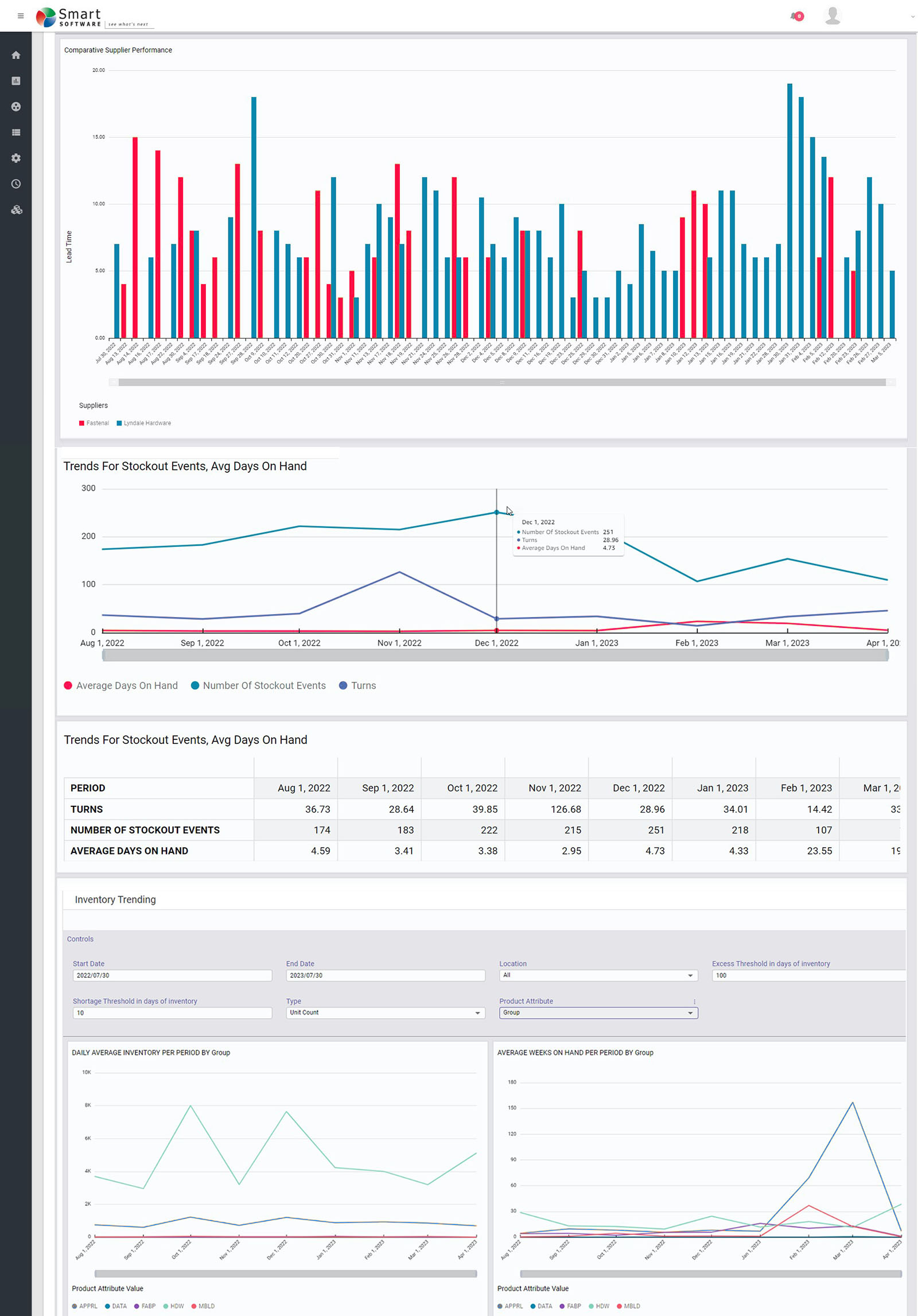
All the calculations guided by the planners using our software ultimately get distilled into the SOA reports for management. The reports focus on five areas: inventory analysis, inventory performance, inventory trending, supplier performance, and demand anomalies.

Inventory Analysis

These reports keep tabs on current inventory levels and identify areas that need improvement. The focus is on current inventory counts and their status (on hand, in transit, in quarantine), inventory turns, and excesses vs shortages.

Inventory Performance

These reports track Key Performance Indicators (KPIs) such as Fill Rates, Service Levels, and inventory Costs. The analytic calculations elsewhere in the software guide you toward achieving your KPI targets by calculating Key Performance Predictions (KPPs) based on recommended settings for, e.g., reorder points and order quantities. But sometimes surprises occur, or operating policies are not executed as recommended, so there will always be some slippage between KPPs and KPIs.

Inventory Trending

Knowing where things stand today is important, but seeing where things are trending is also valuable. These reports reveal trends in item demand, stockout events, average days on hand, average time to ship, and more.

Supplier Performance

Your company cannot perform at its best if your suppliers are dragging you down. These reports monitor supplier performance in terms of the accuracy and promptness of filling replenishment orders. Where you have multiple suppliers for the same item, they let you compare them.

Demand Anomalies

Your entire inventory system is demand driven, and all inventory control parameters are computed after modeling item demand. So if something odd is happening on the demand side, you must be vigilant and prepare to recalculate things like mins and maxes for items that are starting to act in odd ways.

Summary

The end point for all the massive calculations in our software is the dashboard showing management what’s going on, what’s next, and where to focus attention. Smart Inventory Analytics is the part of our software ecosystem aimed at your company’s C-Suite.

 

Figure 1: Some sample reports in graphical form

 

Dealing with the day-to-day of inventory management can keep you busy. There’s the usual rhythm of ordering, receiving, forecasting and planning, and moving things around in the warehouse. Then there are the frenetic times – shortages, expedites, last-minute calls to find new suppliers.

All this activity works against taking a moment to see how you’re doing. But you know you have to get your head up now and then to see where you’re heading. For that, your inventory software should show you metrics – and not just one, but a full set of metrics or KPI’s – Key Performance Indicators.

Multiple Metrics

Depending on your role in your organization, different metrics will have different salience. If you are on the finance side of the house, inventory investment may be top of mind: how much cash is tied up in inventory? If you’re on the sales side, item availability may be top of mind: what’s the chance that I can say “yes” to an order? If you’re responsible for replenishment, how many PO’s will your people have to cut in the next quarter?

Availability Metrics

Let’s circle back to item availability. How do you put a number on that? The two most used availability metrics are “service level” and “fill rate.” What’s the difference? It’s the difference between saying “We had an earthquake yesterday” and saying, “We had an earthquake yesterday, and it was a 6.4 on the Richter scale.” Service level records the frequency of stockouts no matter their size; fill rate reflects their severity. The two can seem to point in opposite directions, which causes some confusion. You can have a good service level, say 90%, but have an embarrassing fill rate, say 50%. Or vice versa. What makes them different is the distribution of demand sizes. For instance, if the distribution is very skewed, so most demands are small but some are huge, you might get the 90%/50% split mentioned above. If your focus is on how often you have to backorder, service level is more relevant. If your worry is how big an overnight expedite can get, the fill rate is more relevant.

One Graph to Rule them All

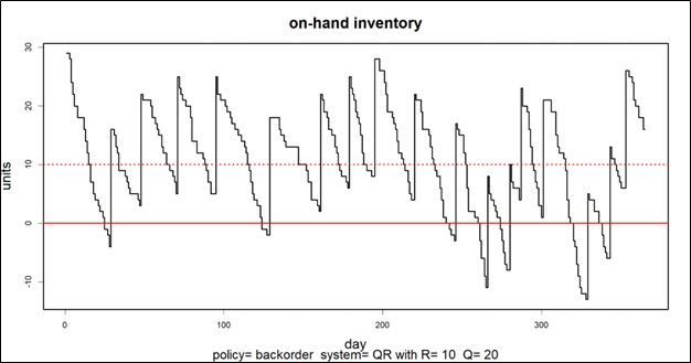
A graph of on-hand inventory can provide the basis for calculating multiple KPI’s. Consider Figure 1, which plots on-hand each day for a year. This plot has information needed to calculate multiple metrics: inventory investment, service level, fill rate, reorder rate and other metrics.

Inventory investment: The average height of the graph when above zero, when multiplied by unit cost of the inventory item, gives quarterly dollar value.

Service level: The fraction of inventory cycles that end above zero is the service level. Inventory cycles are marked by the up movements occasioned by the arrival of replenishment orders.

Fill rate: The amount by which inventory drops below zero and how long it stays there combine to determine fill rate.

In this case, the average number of units on hand was 10.74, the service level was 54%, and the fill rate was 91%.

 

KPI’s and KPP’s

In the over forty years since we founded Smart Software, I have never seen a customer produce a plot like Figure 1.  Those who are further along in their development do produce and pay attention to reports listing their KPI’s in tabular form, but they don’t look at such a graph. Nevertheless, that graph has value for developing insight into the random rhythms of inventory as it rises and falls.

Where it is especially useful is prospectively. Given market volatility, key variables like supplier lead times, average demand, and demand variability all shift over time. This implies that key control parameters like reorder points and order quantities must adjust to these shifts. For instance, if a supplier says they’ll have to increase their average lead time by 2 days, this will impact your metrics negatively, and you may need to increase your reorder point to compensate. But increase it by how much?

Here is where modern inventory software comes in. It will let you propose an adjustment and then see how things will play out. Plots like Figure 1 let you see and get a feel for the new regime. And the plots can be analyzed to compute KPP’s – Key Performance Predictions.

KPP’s help take the guesswork out of adjustments. You can simulate what will happen to your KPI’s if you change them in response to changes in your operating environment – and how bad things will get if you make no changes.

 

 

 

 

Are you confused about what is AI and what is machine learning? Are you unsure why knowing more will help you with your job in inventory planning? Don’t despair. You’ll be ok, and we’ll show you how some of whatever-it-is can be useful.

What is and what isn’t

What is AI and how does it differ from ML? Well, what does anybody do these days when they want to know something? They Google it. And when they do, the confusion starts.

One source says that the neural net methodology called deep learning is a subset of machine learning, which is a subset of AI. But another source says that deep learning is already a part of AI because it sort of mimics the way the human mind works, while machine learning doesn’t try to do that.

One source says there are two types of machine learning: supervised and unsupervised. Another says there are four: supervised, unsupervised, semi-supervised and reinforcement.

Some say reinforcement learning is machine learning; others call it AI.

Some of us traditionalists call a lot of it “statistics”, though not all of it is.

In the naming of methods, there is a lot of room for both emotion and salesmanship. If a software vendor thinks you want to hear the phrase “AI”, they may well say it for you just to make you happy.

Better to focus on what comes out at the end

You can avoid some confusing hype if you focus on the end result you get from some analytic technology, regardless of its label. There are several analytical tasks that are relevant to inventory planners and demand planners. These include clustering, anomaly detection, regime change detection, and regression analysis. All four methods are usually, but not always, classified as machine learning methods. But their algorithms can come straight out of classical statistics.

Clustering

Clustering means grouping together things that are similar and distancing them from things that are dissimilar. Sometimes clustering is easy: to separate your customers geographically, simply sort them by state or sales region. When the problem is not so dead obvious, you can use data and clustering algorithms to get the job done automatically even when dealing with massive datasets.

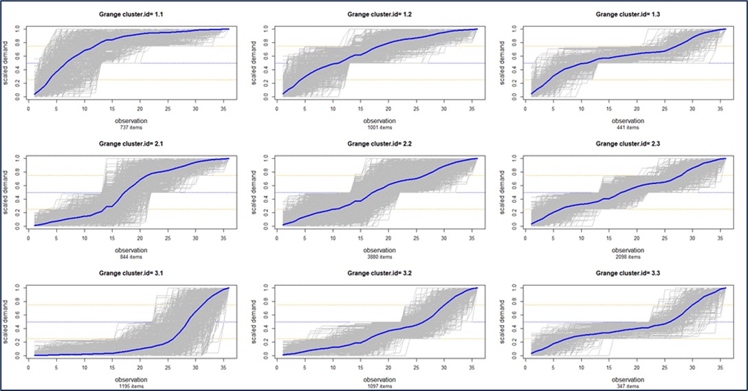
For example, Figure 1 illustrates a cluster of “demand profiles”, which in this case divides all a customer’s items into nine clusters based on the shape of their cumulative demand curves. Cluster 1.1 in the top left contains items whose demand has been petering out, while Cluster 3.1 in the bottom left contains items whose demand has accelerated.  Clustering can also be done on suppliers. The choice of number of clusters is typically left to user judgement, but ML can guide that choice.  For example, a user might instruct the software to “break my parts into 4 clusters” but using ML may reveal that there are really 6 distinct clusters the user should analyze. 

 

Figure 1: Clustering items based on the shapes of their cumulative demand

Anomaly Detection

Demand forecasting is traditionally done using time series extrapolation. For instance, simple exponential smoothing works to find the “middle” of the demand distribution at any time and project that level forward. However, if there has been a sudden, one-time jump up or down in demand in the recent past, that anomalous value can have a significant but unwelcome effect on the near-term forecast.  Just as serious for inventory planning, the anomaly can have an outsized effect on the estimate of demand variability, which goes directly to the calculation of safety stock requirements.

Planners may prefer to find and remove such anomalies (and maybe do offline follow-up to find out the reason for the weirdness). But nobody with a big job to do will want to visually scan thousands of demand plots to spot outliers, expunge them from the demand history, then recalculate everything. Human intelligence could do that, but human patience would soon fail. Anomaly detection algorithms could do the work automatically using relatively straightforward statistical methods. You could call this “artificial intelligence” if you wish.

Regime Change Detection

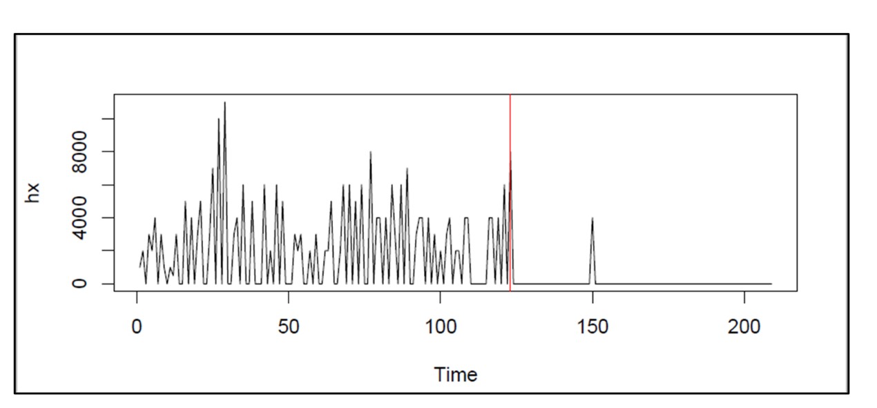
Regime change detection is like the big brother of anomaly detection. Regime change is a sustained, rather than temporary, shift in one or more aspects of the character of a time series. While anomaly detection usually focuses on sudden shifts in mean demand, regime change could involve shifts in other features of the demand, such as its volatility or its distributional shape.  

Figure 2 illustrates an extreme example of regime change. The bottom dropped out of demand for this item around day 120. Inventory control policies and demand forecasts based on the older data would be wildly off base at the end of the demand history.

Figure 2: An example of extreme regime change in an item with intermittent demand

Here too, statistical algorithms can be developed to solve this problem, and it would be fair play to call them “machine learning” or “artificial intelligence” if so motivated.  Using ML or AI to identify regime changes in demand history enables demand planning software to automatically use only the relevant history when forecasting instead of having to manually pick the amount of history to introduce to the model. 

Regression analysis

Regression analysis relates one variable to another through an equation. For example, sales of window frames in one month may be predicted from building permits issued a few months earlier. Regression analysis has been considered a part of statistics for over a century, but we can say it is “machine learning” since an algorithm works out the precise way to convert knowledge of one variable into a prediction of the value of another.

Summary

It is reasonable to be interested in what’s going on in the areas of machine learning and artificial intelligence. While the attention given to ChatGPT and its competitors is interesting, it is not relevant to the numerical side of demand planning or inventory management. The numerical aspects of ML and AI are potentially relevant, but you should try to see through the cloud of hype surrounding these methods and focus on what they can do.  If you can get the job done with classical statistical methods, you might just do that, then exercise your option to stick the ML label on anything that moves.