Reveal how forecasts are used with these 4 questions.

Often companies will insist that they “don’t use forecasts” to plan inventory.  They often use reorder point methods and are struggling to improve on-time delivery, inventory turns, and other KPIs. While they don’t think of what they are doing as explicitly forecasting, they certainly use estimates of future demand to develop reorder points such as min/max.

Regardless of what it is called, everyone tries to estimate future demand in some way and uses this estimate to set stocking policies and drive orders. To improve inventory planning and make sure you aren’t over/under ordering and creating large stockouts and inventory bloat, it is important to understand exactly how your organization uses forecasts. Once this is understood, you can assess whether the quality of the forecasts can be improved.

Try getting answers to the following questions. It will reveal how forecasts are being used in your business – even if you don’t think you use forecasts.

1.  Is your forecast a period-by-period estimate over time that is used to predict what on-hand inventory will be in the future and triggers order suggestions in your ERP system?

2. Or is your forecast used to derive a reorder point but not explicitly used as a per-period driver to trigger orders? Here, I may predict we’ll sell 10 per week based on the history, but we are not loading 10, 10, 10, 10, etc., into the ERP. Instead, I derive a reorder point or Min that covers the two-period lead time + some amount of buffer to help protect against stock out. In this case, I’ll order more when on hand gets to 25.

3. Is your forecast used as a guide for the planner to help subjectively determine when they should order more?  Here, I predict 10 per week, and I assess the on-hand inventory periodically, review the expected lead time, and I decide, given the 40 units I have on hand today, that I have “enough.” So, I do nothing now but will check back again in a week.

4. Is it used to set up blanket orders with suppliers? Here, I predict 10 per week and agree to a blanket purchase order with the supplier of 520 per year. The orders are then placed in advance to arrive in quantities of 10 once per week until the blanket order is consumed.

Once you get the answers, you can then ask how the estimates of demand are created.  Is it an average? Is it deriving demand over lead time from a sales forecast?  Is there a statistical forecast generated somewhere?  What methods are considered? It will also be important to assess how safety stocks are used to protect against demand and supply variability.  More on all of this in a future article.

Every organization that runs equipment needs spare parts. All of them must cope with issues that are generic no matter what their business. Some of the problems, however, are industry specific. This post discusses one universal problem that manifested in a nuclear plant and one that is especially acute for any electric utility.

The Universal Problem of Data Quality

We often post about the benefits of converting parts usage data into smart inventory management decisions. Advanced probability modeling supports generation of realistic demand scenarios that feed into detailed Monte Carlo simulations that expose the consequences of decisions such as choices of Min and Max governing the replenishment of spares.

However, all that new and shiny analytical tech requires quality data as fuel for the analysis. For some public utilities of all kinds, record keeping is not a strong suit, so the raw material going into analysis can be corrupted and misleading. We recently chanced upon documentation of a stark example of this problem at a nuclear power plant (see Scala, ­­­­­­­Needy and Rajgopal: Decision making and tradeoffs in the management of spare parts inventory at utilities. American Association of Engineering Management, 30th ASEM National Conference, Springfield, MO. October 2009). Scala et al. documented the usage history of a critical part whose absence would result in either a facility de-rate or a shutdown. The plant’s usage record for that part spanned more than eight years of data. During that time, the official usage history reported nine events in which positive demand occurred with sizes ranging from one to six units each. There were also five events marked by negative demands (i.e., returns to warehouse) ranging from one to three units each. Careful sleuthing discovered that the true usage occurred in just two events, both with demand of two units. Obviously, calculating the best Min/Max values for this item requires accurate demand data.

The Special Problem of Health and Safety

In the context of “regular” businesses, shortages of spare parts can damage both current revenue and future revenue (related to reputation as a reliable supplier). For an electric utility, however, Scala et al. noted a much greater level of consequence attached to stockouts of spare parts. These include not only a heightened financial and reputational risk but also risks to health and safety: “Ramifications of not having a part in stock include the possibility of having to reduce output or quite possibly, even a plant shut down. From a more long-term perspective, doing so might interrupt the critical service of power to residential, commercial, and/or industrial customers, while damaging the company’s reputation, reliability, and profitability. An electric utility makes and sells only one product: electricity. Losing the ability to sell electricity can be seriously damaging to the company’s bottom line as well its long-term viability.”

All the more reason for electric utilities to be leaders rather than laggards in the deployment of the most advanced probability models for demand forecasting and inventory optimization.

Outside of work, you may have heard the famous dictum “Correlation is not causation.” It may sound like a piece of theoretical fluff that, though involved in a recent Noble Prize in economics, isn’t relevant to your work as a demand planner. Is so, you may be only partially correct.

Extrapolative vs Causal Models

Most demand forecasting uses extrapolative models. Also called time-series models, these forecast demand using only the past values of an item’s demand. Plots of past values reveal trend and seasonality and volatility, so there is a lot they are good for. But there is another type of model – causal models —that can potentially improve forecast accuracy beyond what you can get from extrapolative models.

Causal models bring more input data to the forecasting task: information on presumed forecast “drivers” external to the demand history of an item. Examples of potentially useful causal factors include macroeconomic variables like the inflation rate, the rate of GDP growth, and raw material prices. Examples not tied to the national economy include industry-specific growth rates and your own and competitors’ ad spending.  These variables are usually used as inputs to regression models, which are equations with demand as an output and causal variables as inputs.

Forecasting using Causal Models

Many firms have an S&OP process that involves a monthly review of statistical (extrapolative) forecasts in which management adjusts forecasts based on their judgement. Often this is an indirect and subjective way to work causal models into the process without doing the regression modeling.

To actually make a causal regression model, first you have to nominate a list of potentially-useful causal predictor variables. These may come from your subject matter expertise. For example, suppose you manufacture window glass. Much of your glass may end up in new homes and new office buildings. So, the number of new homes and offices being built are plausible predictor variables in a regression equation.

There is a complication here: if you are using the equation to predict something, you must first predict the predictors. For example, sales of glass next quarter may be strongly related to numbers of new homes and new office buildings next quarter. But how many new homes will there be next quarter? That’s its own forecasting problem. So, you have a potentially powerful forecasting model, but you have extra work to do to make it usable.

There is one way to simplify things: if the predictor variables are “lagged” versions of themselves. For example, the number of new building permits issued six months ago may be a good predictor of glass sales next month. You don’t have to predict the building permit data – you just have to look it up.

Is it a causal relationship or just a spurious correlation?

Causal models are the real deal: there is an actual mechanism that relates the predictor variable to the predicted variable. The example of predicting glass sales from building permits is an example.

A correlation relationship is more iffy. There is a statistical association that may or may not provide a solid basis for forecasting. For example, suppose you sell a product that happens to appeal most strongly to Dutch people but you don’t realize this. The Dutch are, on average, the tallest people in Europe. If your sales are increasing and the average height of Europeans is increasing, you might use that relationship to good effect. However, if the proportion of Dutch in the Euro zone is decreasing while the average height is increasing because the mix of men versus women is shifting toward men, what can go wrong? You will expect sales to increase because average height is increasing. But your sales are really mostly to the Dutch, and their relative share of the population is shrinking, so your sales are really going to decrease instead. In this case the association between sales and customer height is a spurious correlation.

How can you tell the difference between true and spurious relationships? The gold standard is to do a rigorous scientific experiment. But you are not likely to be in position to do that. Instead, you have to rely on your personal “mental model” of how your market works. If your hunches are right, then your potential causal models will correlate with demand and causal modeling will pay off for you, either to supplement extrapolative models or to replace them.

Forecast accuracy is a key metric by which to judge the quality of your demand planning process. (It’s not the only one. Others include timeliness and cost; See 5 Demand Planning Tips for Calculating Forecast Uncertainty.) Once you have forecasts, there are a number of ways to summarize their accuracy, usually designated by obscure three- or four-letter acronyms like MAPE, RMSE, and MAE.  See Four Useful Ways to Measure Forecast Error for more detail.

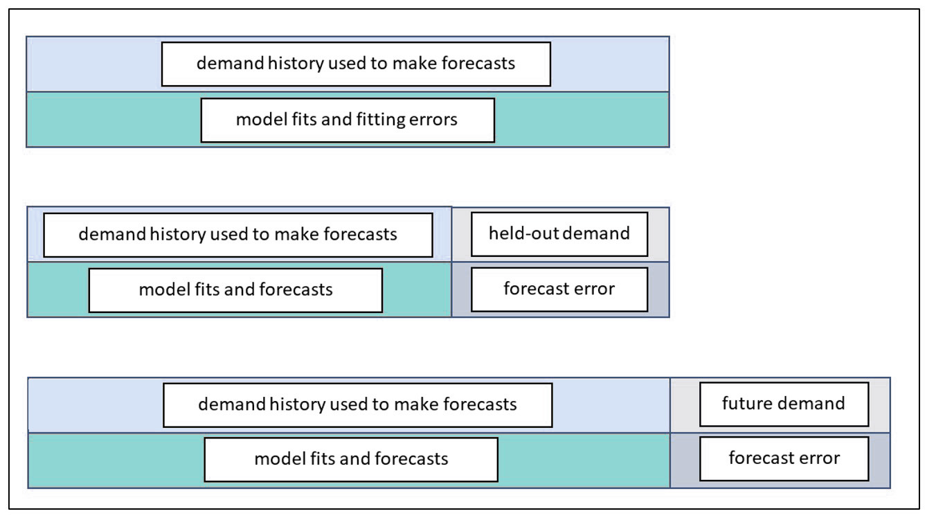
A less discussed but more fundamental issue is how computational experiments are organized for computing forecast error. This post compares the three most important experimental designs. One of them is old-school and essentially amounts to cheating. Another is the gold standard. A third is a useful expedient that mimics the gold standard and is best thought of as predicting how the gold standard will turn out. Figure 1 is a schematic view of the three methods.

Figure 1: Three ways to assess forecast error

The top panel of Figure 1 depicts the way forecast error was assessed back in the early 1980’s before we moved the state of the art to the scheme shown in the middle panel. In the old days, forecasts were assessed on the same data used to compute the forecasts. After a model was fit to the data, the errors computed were not for model forecasts but for model fits. The difference is that forecasts are for future values, while fits are for concurrent values. For example, suppose the forecasting model is a simple moving average of the three most recent observations. At time 3, the model computes the average of observations 1, 2, and 3. This average would then be compared to the observed value at time 3. We call this cheating because the observed value at time 3 got a vote on what the forecast should be at time 3. A true forecast assessment would compare the average of the first three observations to the value of the next, fourth, observation. Otherwise, the forecaster is left with an overly optimistic assessment of forecast accuracy.

The bottom panel of Figure 1 shows the best way to assess forecast accuracy. In this schema, all the historical demand data are used to fit a model, which is then used to forecast future, unknown demand values. Eventually, the future unfolds, the true future values reveal themselves, and actual forecast errors can be computed. This is the gold standard. This information populates the “forecasts versus actuals” report in our software.

The middle panel depicts a useful halfway measure. The problem with the gold standard is that you must wait to learn how well your chosen forecasting methods perform. This delay does not help when you are required to choose, in the moment, which forecasting method to use for each item. Nor does it provide a timely estimate of the forecast uncertainty you will experience, which is important for risk management such as forecast hedging. The middle way is based on hold-out analysis, which excludes (“holds out”) the most recent observations and asks the forecasting method to do its work without knowing those ground truths. Then the forecasts based on the foreshortened demand history can be compared to the held-out actual values to get an honest assessment of forecast error.

​If you had your head up lately, you may have noticed some additional madness off the basketball court: The failure of Silicon Valley Bank. Those of us in the supply chain world may have dismissed the bank failure as somebody else’s problem, but that sorry episode holds a big lesson for us, too: The importance of stress testing done right.

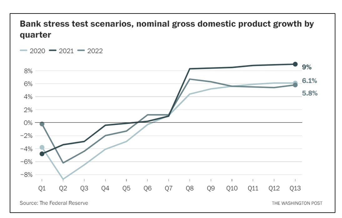
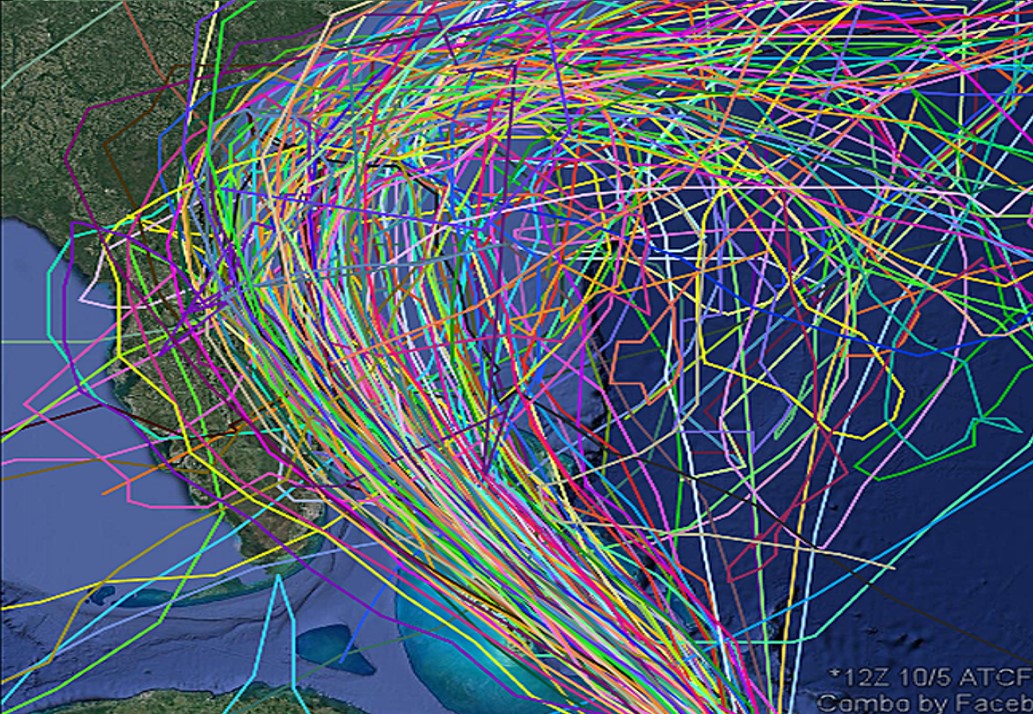
The Washington Post recently carried an opinion piece by Natasha Sarin called “Regulators missed Silicon Valley Bank’s problems for months. Here’s why.” Sarin outlined the flaws in the stress testing regime imposed on the bank by the Federal Reserve. One problem is that the stress tests are too static. The Fed’s stress factor for nominal GDP growth was a single scenario listing presumed values over the next 13 quarters (see Figure 1). Those 13 quarterly projections might be somebody’s consensus view of what a bad hair day would look like, but that’s not the only way things could play out.  As a society, we are being taught to appreciate a better way to display contingencies every time the National Weather Service shows us projected hurricane tracks (see Figure 2). Each scenario represented by a different colored line shows a possible storm path, with the concentrated lines representing the most likely.  By exposing the lower probability paths, risk planning is improved.

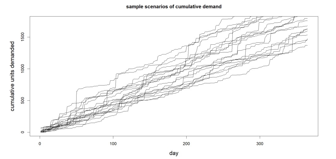
When stress testing the supply chain, we need realistic scenarios of possible future demands that might occur, even extreme demands.   Smart provides this in our software (with considerable improvements in our Gen2 methods).  The software generates a huge number of credible demand scenarios, enough to expose the full scope of risks (see Figure 3). Stress testing is all about generating massive numbers of planning scenarios, and Smart’s probabilistic methods are a radical departure from previous deterministic S&OP applications, being entirely scenario based.

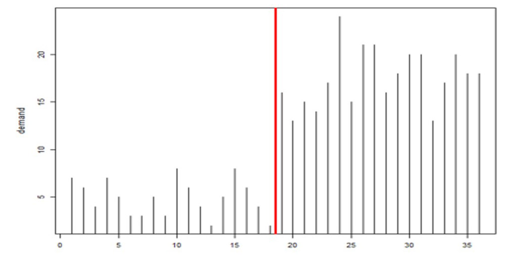
The other flaw in the Fed’s stress tests was that they were designed months in advance but never updated for changing conditions.  Demand planners and inventory managers intuitively appreciate that key variables like item demand and supplier lead time are not only highly random even when things are stable but also subject to abrupt shifts that should require rapid rewriting of planning scenarios (see Figure 4, where the average demand jumps up dramatically between observations 19 and 20). Smart’s Gen2 products include new tech for detecting such “regime changes”  and automatically changing scenarios accordingly.

Banks are forced to undergo stress tests, however flawed they may be, to protect their depositors. Supply chain professionals now have a way to protect their supply chains by using modern software to stress test their demand plans and inventory management decisions.

Figure 1: Scenarios used the Fed to stress test banks.

Figure 2: Scenarios used by the National Weather Service to predict hurricane tracks

Figure 3: Demand scenarios of the type generated by Smart Demand Planner

Figure 4: Example of regime change in product demand after observation #19