Some companies invest in software to help them manage their inventory, whether it’s spare parts or finished goods. But a surprising number of others play the Inventory Guessing Game every day, trusting to an imagined “Golden Gut” or to plain luck to set their inventory control parameters. But what kind of results do you expect with that approach?

How good are you at intuiting the right values? This blog post challenges you to guess the best Min and Max values for a notional inventory item. We’ll show you its demand history, give you a few relevant facts, then you can pick Min and Max values and see how well they would work. Ready?

The Challenge

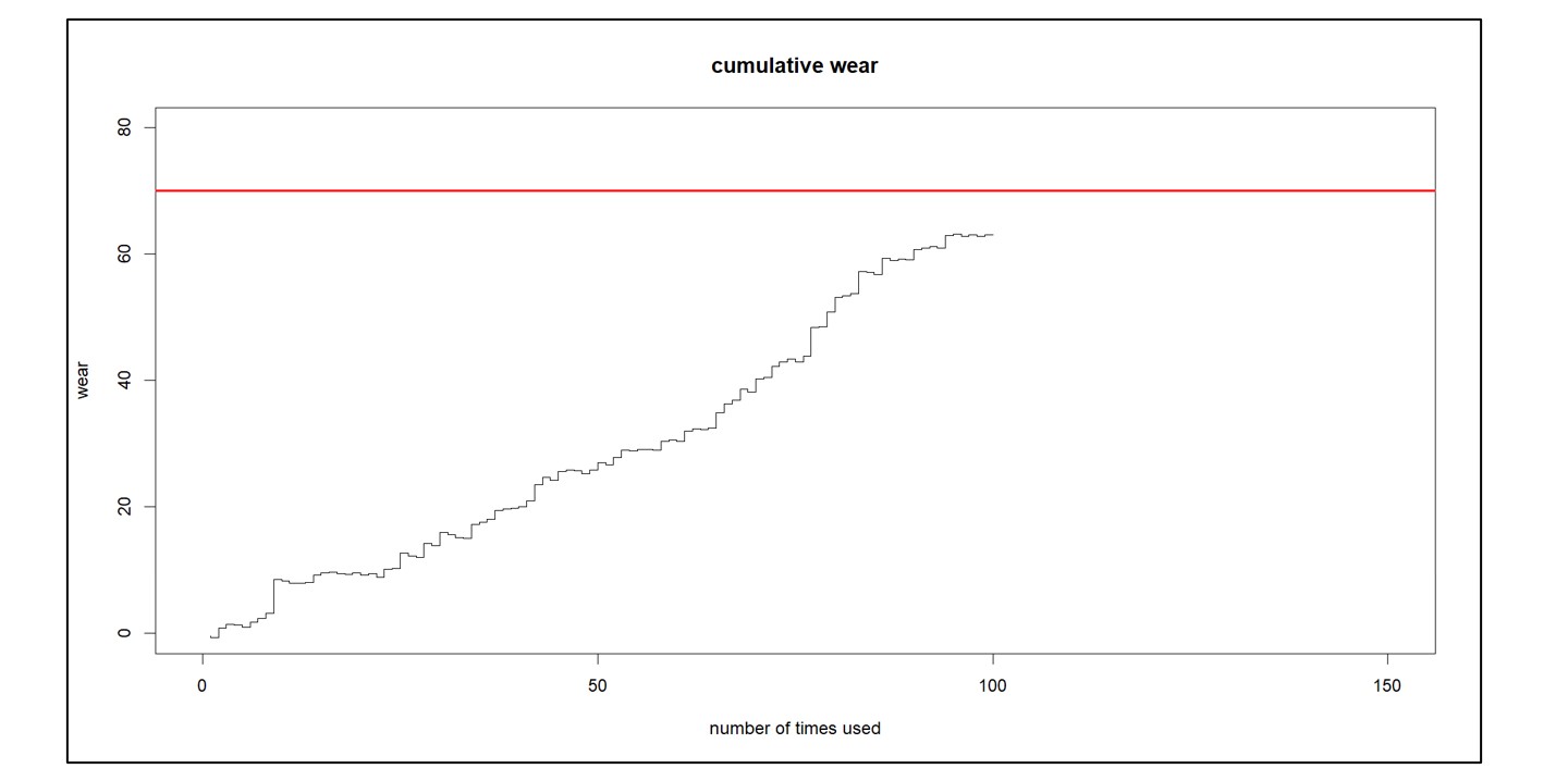
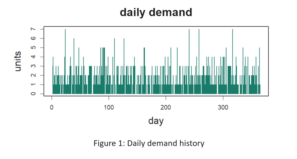
Figure 1 shows the daily demand history of the item. The average demand is 2 units per day. Replenishment lead time is a constant 10 days (which is unrealistic but works in your favor). Orders that cannot be filled immediately from stock cannot be backordered and are lost. You want to achieve at least an 80% fill rate, but not at any cost. You also want to minimize the average number of units on hand while still achieving at least an 80% fill rate. What Min and Max values would produce an 80% fill rate with the lowest average number of units on hand? [Record your answers for checking later. The solution appears below at the end of the article.]

Computing the Best Min and Max Values

The way to determine the best values is to use a digital twin, also known as a Monte Carlo simulation. The analysis creates a multitude of demand scenarios and passes them through the mathematical logic of the inventory control system to see what values will be taken on by key performance indicators (KPI’s).

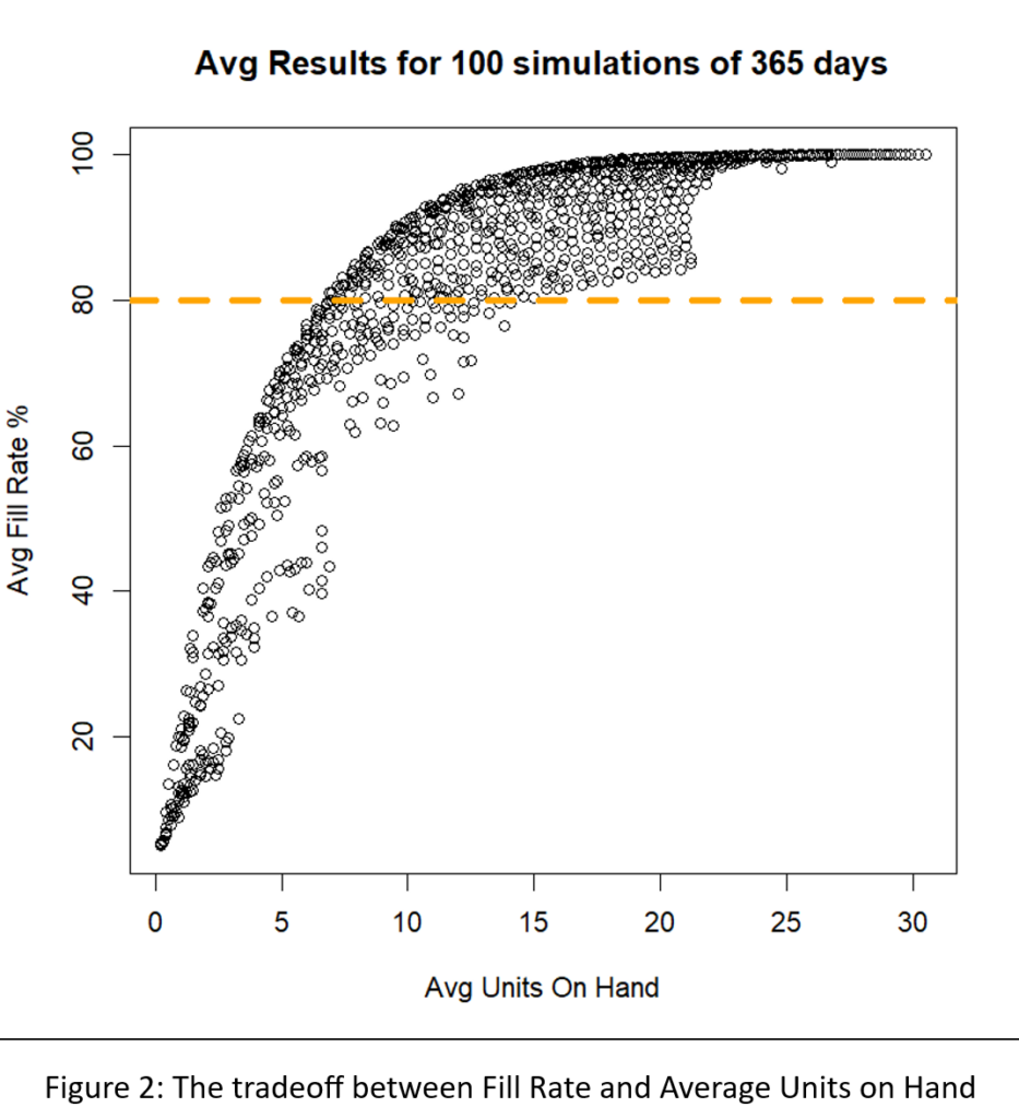
We built a digital twin for this problem and systematically exercised it with 1,085 pairs of Min and Max values. For each pair, we simulated 365 days of operation a total of 100 times. Then we averaged the results to assess the performance of the Min/Max pair in terms of two KPI’s: fill rate and average on hand inventory.

Figure 2 shows the results. The inherent tradeoff between inventory size and fill rate is clear in the figure: if you want a higher fill rate, you have to accept a larger inventory. However, at each level of inventory there is a range of fill rates, so the game is to find the Min/Max pair that yields the highest fill rate for any given size inventory.

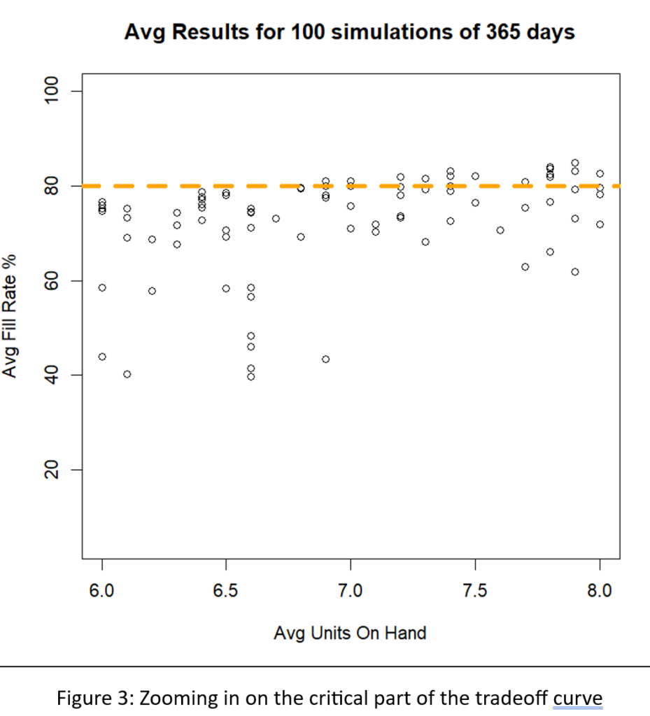
A different way to interpret Figure 2 is to focus on the dashed green line marking the target 80% fill rate. There are many Min/Max pairs that can hit near the 80% target, but they differ in inventory size from about 6 to about 8 units. Figure 3 zooms in on that region of Figure 2 to show  quite a number of Min/Max pairs that are competitive.

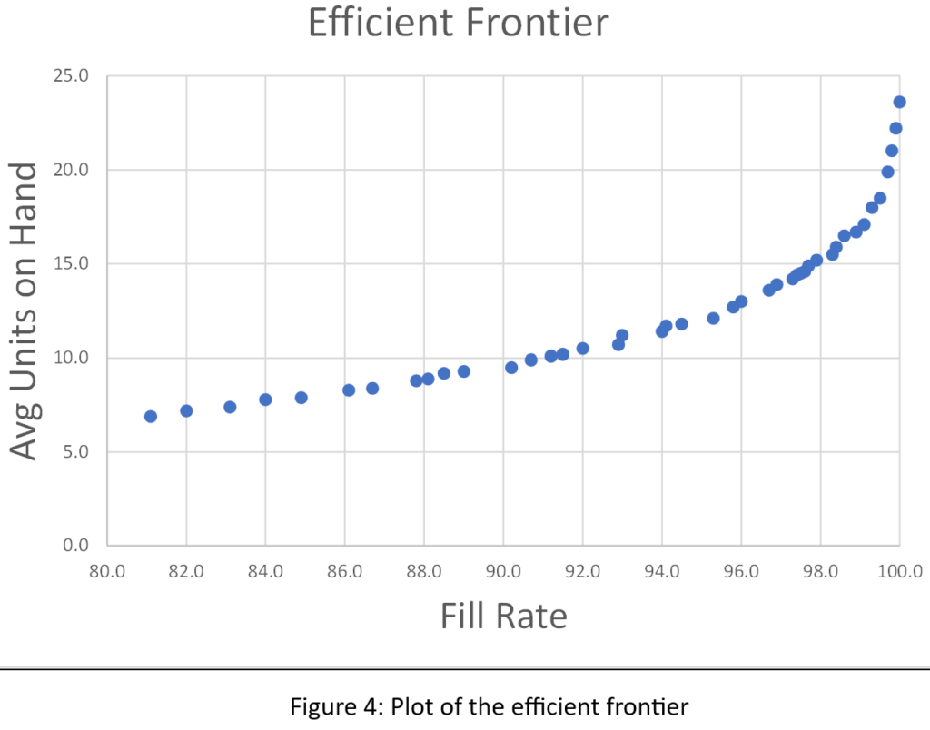
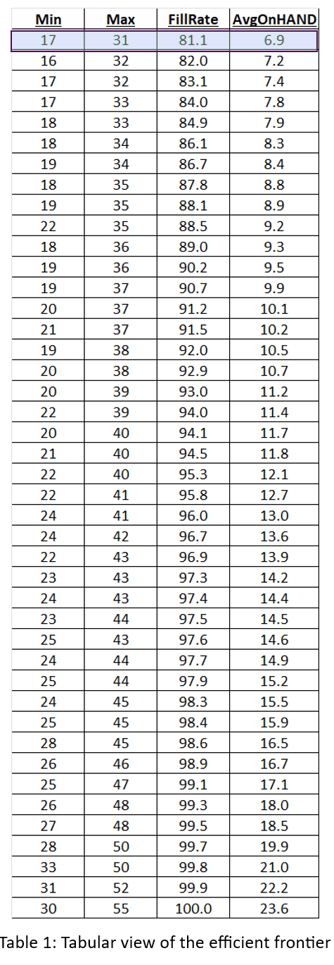
We sorted the results of all 1,085 simulations to identify what economists call the efficient frontier. The efficient frontier is the set of most efficient Min/Max pairs to exploit the tradeoff between fill rate and units on hand. That is, it is a list of Min/Max pairs that provide the least cost way to achieve any desired fill rate, not just 80%. Figure 4 shows the efficient frontier for this problem. Moving from left to right, you can read off the lowest price you would have to pay (as measured by average inventory size) to achieve any target fill rate. For example, to achieve a 90% fill rate, you would have to carry an average inventory of about 10 units.

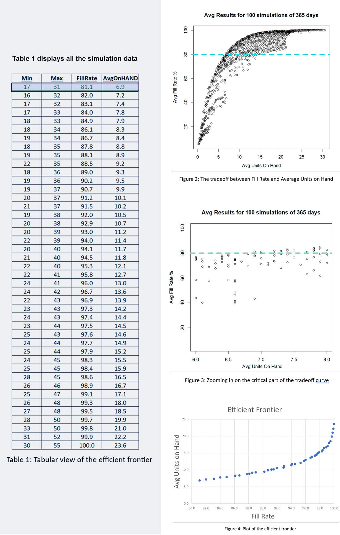
Figures 2, 3, and 4 show results for various Min/Max pairs but do not display the values of Min and Max behind each point. Table 1 displays all the simulation data: the values of Min, Max, average units on hand and fill rate. The answer to the guessing game is highlighted in the first line of the table: Min=7 and Max=13¹. Did you get the right answer, or something close²? Did you maybe get onto the efficient frontier?

Conclusions

Maybe you got lucky, or maybe you do indeed have a Golden Gut, but it’s more likely you didn’t get the right answer, and it’s even more likely you didn’t even try. Figuring out the right answer is extremely difficult without using the digital twin. Guessing is unprofessional.

One step up from guessing is “guess and see”, in which you implement your guess and then wait a while (months?) to see if you like the results. That tactic is at least “scientific”, but it is inefficient.

Now consider the effort to work out the best (Min,Max) pairs for thousands of items. At that scale, there is even less justification for playing the Inventory Guessing Game. The right answer is to play it… Smart³.

¹ This answer has a bonus, in that it achieves a bit more than 80% fill rate at a lower average inventory size than the Min/Max combination that hit exactly 80%. In other words, (7,13) is on the efficient frontier.

² Because these results come from a simulation instead of an exact mathematical equation, there is a certain margin of error associated with each estimated fill rate and inventory level. However, because the average results were based on 100 simulations each 365 days long, the margins of error are small. Across all experiments, the average standard errors in fill rate and mean inventory were, respectively, only 0.009% and 0.129 units.

³ In case you didn’t know this, one of the founders of Smart Software was … Charlie Smart.

I’ll start with a confession: I’m an algorithm guy. My heart lives in the “engine room” of our software, where lightning-fast calculations zip back and forth across the AWS cloud, generating demand and supply scenarios used to guide important decisions about demand forecasting and inventory management.

But I recognize that the target of all that beautiful, furious calculation is the brain of the boss, the person responsible for making sure that customer demand is satisfied in the most efficient and profitable way. So, this blog is about Smart Operational Analytics (SOA), which creates reports for management. Or, as they are called in the military, sit-reps.

All the calculations guided by the planners using our software ultimately get distilled into the SOA reports for management. The reports focus on five areas: inventory analysis, inventory performance, inventory trending, supplier performance, and demand anomalies.

Inventory Analysis

These reports keep tabs on current inventory levels and identify areas that need improvement. The focus is on current inventory counts and their status (on hand, in transit, in quarantine), inventory turns, and excesses vs shortages.

Inventory Performance

These reports track Key Performance Indicators (KPIs) such as Fill Rates, Service Levels, and inventory Costs. The analytic calculations elsewhere in the software guide you toward achieving your KPI targets by calculating Key Performance Predictions (KPPs) based on recommended settings for, e.g., reorder points and order quantities. But sometimes surprises occur, or operating policies are not executed as recommended, so there will always be some slippage between KPPs and KPIs.

Inventory Trending

Knowing where things stand today is important, but seeing where things are trending is also valuable. These reports reveal trends in item demand, stockout events, average days on hand, average time to ship, and more.

Supplier Performance

Your company cannot perform at its best if your suppliers are dragging you down. These reports monitor supplier performance in terms of the accuracy and promptness of filling replenishment orders. Where you have multiple suppliers for the same item, they let you compare them.

Demand Anomalies

Your entire inventory system is demand driven, and all inventory control parameters are computed after modeling item demand. So if something odd is happening on the demand side, you must be vigilant and prepare to recalculate things like mins and maxes for items that are starting to act in odd ways.

Summary

The end point for all the massive calculations in our software is the dashboard showing management what’s going on, what’s next, and where to focus attention. Smart Inventory Analytics is the part of our software ecosystem aimed at your company’s C-Suite.

Figure 1: Some sample reports in graphical form

What’s different about inventory planning for Maintenance, Repair, and Operations (MRO) compared to inventory planning in manufacturing and distribution environments? In short, it’s the nature of the demand patterns combined with the lack of actionable business knowledge.

Demand Patterns

Manufacturers and distributors tend to focus on the top sellers that generate the majority of their revenue. These items typically have high demand that is relatively easy to forecast with traditional time series models that capitalize on predictable trend and/or seasonality.  In contrast, MRO planners almost always deal with intermittent demand, which is more sparse, more random, and harder to forecast.  Furthermore, the fundamental quantities of interest are different. MRO planners ultimately care most about the “when” question:  When will something break? Whereas the others focus on the “how much” question of units sold.

Business Knowledge

Manufacturing and distribution planners can often count on gathering customer and sales feedback, which can be combined with statistical methods to improve forecast accuracy. On the other hand, bearings, gears, consumable parts, and repairable parts are rarely willing to share their opinions. With MRO, business knowledge about which parts will be needed and when just isn’t reliable (excepting planned maintenance when higher-volume consumable parts are replaced). So, MRO inventory planning success goes only as far as their probability models’ ability to predict future usage takes them. And since demand is so intermittent, they can’t get past Go with traditional approaches.

Methods for MRO

In practice, it is common for MRO and asset-intensive businesses to manage inventories by resorting to static Min/Max levels based on subjective multiples of average usage, supplemented by occasional manual overrides based on gut feel. The process becomes a bad mixture of static and reactive, with the result that a lot of time and money is wasted on expediting.

There are alternative planning methods based more on math and data, though this style of planning is less common in MRO than in the other domains. There are two leading approaches to modeling part and machine breakdown: models based on reliability theory and “condition-based maintenance” models based on real-time monitoring.

Reliability Models

Reliability models are the simpler of the two and require less data. They assume that all items of the same type, say a certain spare part, are statistically equivalent. Their key component is a “hazard function”, which describes the risk of failure in the next little interval of time. The hazard function can be translated into something better suited for decision making: the “survival function”, which is the probability that the item is still working after X amount of use (where X might be expressed in days, months, miles, uses, etc.). Figure 1 shows a constant hazard function and its corresponding survival function.

Figure 1: Constant hazard function and its survival function

A hazard function that doesn’t change implies that only random accidents will cause a failure. In contrast, a hazard function that increases over time implies that the item is wearing out. And a decreasing hazard function implies that an item is settling in. Figure 2 shows an increasing hazard function and its corresponding survival function.

Figure 2: Increasing hazard function and its survival function

Reliability models are often used for inexpensive parts, such as mechanical fasteners, whose replacement may be neither difficult nor expensive (but still might be essential).

Condition-Based Maintenance

Models based on real-time monitoring are used to support condition-based maintenance (CBM) for expensive items like jet engines. These models use data from sensors embedded in the items themselves. Such data are usually complex and proprietary, as are the probability models supported by the data. The payoff from real-time monitoring is that you can see trouble coming, i.e., the deterioration is made visible, and forecasts can predict when the item will hit its red line and therefore need to be taken off the field of play. This allows individualized, pro-active maintenance or replacement of the item.

Figure 3 illustrates the kind of data used in CBM. Each time the system is used, there is a contribution to its cumulative wear and tear. (However, note that sometimes use can improve the condition of the unit, as when rain helps keep a piece of machinery cool). You can see the general trend upward toward a red line after which the unit will require maintenance. You can extrapolate the cumulative wear to estimate when it will hit the red line and plan accordingly.

Figure 3: Illustrating real-time monitoring for condition-based maintenance

To my knowledge, nobody makes such models of their finished goods customers to predict when and how much they will next order, perhaps because the customers would object to wearing brain monitors all the time. But CBM, with its complex monitoring and modeling, is gaining in popularity for can’t-fail systems like jet engines. Meanwhile, classical reliability models still have a lot of value for managing large fleets of cheaper but still essential items.

Smart’s approach
The above condition-based maintenance and reliability approaches require an excessive data collection and cleansing burden that many MRO companies are unable to manage. For those companies, Smart offers an approach that does not require development of reliability models. Instead, it exploits usage data in a different way. It leverages probability-based models of both usage and supplier lead times to simulate thousands of possible scenarios for replenishment lead times and demand.  The result is an accurate distribution of demand and lead times for each consumable part that can be exploited to determine optimal stocking parameters.   Figure 4 shows a simulation that begins with a scenario for spare part demand (upper plot) then produces a scenario of on-hand supply for particular choices of Min/Max values (lower line). Key Performance Indicators (KPIs) can be estimated by averaging the results of many such simulations.

Figure 4: An example of a simulation of spare part demand and on-hand inventory

You can read about Smart’s approach to forecasting spare parts here: https://smartcorp.com/wp-content/uploads/2019/10/Probabilistic-Forecasting-for-Intermittent-Demand.pdf

Dealing with the day-to-day of inventory management can keep you busy. There’s the usual rhythm of ordering, receiving, forecasting and planning, and moving things around in the warehouse. Then there are the frenetic times – shortages, expedites, last-minute calls to find new suppliers.

All this activity works against taking a moment to see how you’re doing. But you know you have to get your head up now and then to see where you’re heading. For that, your inventory software should show you metrics – and not just one, but a full set of metrics or KPI’s – Key Performance Indicators.

Multiple Metrics

Depending on your role in your organization, different metrics will have different salience. If you are on the finance side of the house, inventory investment may be top of mind: how much cash is tied up in inventory? If you’re on the sales side, item availability may be top of mind: what’s the chance that I can say “yes” to an order? If you’re responsible for replenishment, how many PO’s will your people have to cut in the next quarter?

Availability Metrics

Let’s circle back to item availability. How do you put a number on that? The two most used availability metrics are “service level” and “fill rate.” What’s the difference? It’s the difference between saying “We had an earthquake yesterday” and saying, “We had an earthquake yesterday, and it was a 6.4 on the Richter scale.” Service level records the frequency of stockouts no matter their size; fill rate reflects their severity. The two can seem to point in opposite directions, which causes some confusion. You can have a good service level, say 90%, but have an embarrassing fill rate, say 50%. Or vice versa. What makes them different is the distribution of demand sizes. For instance, if the distribution is very skewed, so most demands are small but some are huge, you might get the 90%/50% split mentioned above. If your focus is on how often you have to backorder, service level is more relevant. If your worry is how big an overnight expedite can get, the fill rate is more relevant.

One Graph to Rule them All

A graph of on-hand inventory can provide the basis for calculating multiple KPI’s. Consider Figure 1, which plots on-hand each day for a year. This plot has information needed to calculate multiple metrics: inventory investment, service level, fill rate, reorder rate and other metrics.

Inventory investment: The average height of the graph when above zero, when multiplied by unit cost of the inventory item, gives quarterly dollar value.

Service level: The fraction of inventory cycles that end above zero is the service level. Inventory cycles are marked by the up movements occasioned by the arrival of replenishment orders.

Fill rate: The amount by which inventory drops below zero and how long it stays there combine to determine fill rate.

In this case, the average number of units on hand was 10.74, the service level was 54%, and the fill rate was 91%.

KPI’s and KPP’s

In the over forty years since we founded Smart Software, I have never seen a customer produce a plot like Figure 1.  Those who are further along in their development do produce and pay attention to reports listing their KPI’s in tabular form, but they don’t look at such a graph. Nevertheless, that graph has value for developing insight into the random rhythms of inventory as it rises and falls.

Where it is especially useful is prospectively. Given market volatility, key variables like supplier lead times, average demand, and demand variability all shift over time. This implies that key control parameters like reorder points and order quantities must adjust to these shifts. For instance, if a supplier says they’ll have to increase their average lead time by 2 days, this will impact your metrics negatively, and you may need to increase your reorder point to compensate. But increase it by how much?

Here is where modern inventory software comes in. It will let you propose an adjustment and then see how things will play out. Plots like Figure 1 let you see and get a feel for the new regime. And the plots can be analyzed to compute KPP’s – Key Performance Predictions.

KPP’s help take the guesswork out of adjustments. You can simulate what will happen to your KPI’s if you change them in response to changes in your operating environment – and how bad things will get if you make no changes.

Are you confused about what is AI and what is machine learning? Are you unsure why knowing more will help you with your job in inventory planning? Don’t despair. You’ll be ok, and we’ll show you how some of whatever-it-is can be useful.

What is and what isn’t

What is AI and how does it differ from ML? Well, what does anybody do these days when they want to know something? They Google it. And when they do, the confusion starts.

One source says that the neural net methodology called deep learning is a subset of machine learning, which is a subset of AI. But another source says that deep learning is already a part of AI because it sort of mimics the way the human mind works, while machine learning doesn’t try to do that.

One source says there are two types of machine learning: supervised and unsupervised. Another says there are four: supervised, unsupervised, semi-supervised and reinforcement.

Some say reinforcement learning is machine learning; others call it AI.

Some of us traditionalists call a lot of it “statistics”, though not all of it is.

In the naming of methods, there is a lot of room for both emotion and salesmanship. If a software vendor thinks you want to hear the phrase “AI”, they may well say it for you just to make you happy.

Better to focus on what comes out at the end

You can avoid some confusing hype if you focus on the end result you get from some analytic technology, regardless of its label. There are several analytical tasks that are relevant to inventory planners and demand planners. These include clustering, anomaly detection, regime change detection, and regression analysis. All four methods are usually, but not always, classified as machine learning methods. But their algorithms can come straight out of classical statistics.

Clustering

Clustering means grouping together things that are similar and distancing them from things that are dissimilar. Sometimes clustering is easy: to separate your customers geographically, simply sort them by state or sales region. When the problem is not so dead obvious, you can use data and clustering algorithms to get the job done automatically even when dealing with massive datasets.

For example, Figure 1 illustrates a cluster of “demand profiles”, which in this case divides all a customer’s items into nine clusters based on the shape of their cumulative demand curves. Cluster 1.1 in the top left contains items whose demand has been petering out, while Cluster 3.1 in the bottom left contains items whose demand has accelerated.  Clustering can also be done on suppliers. The choice of number of clusters is typically left to user judgement, but ML can guide that choice.  For example, a user might instruct the software to “break my parts into 4 clusters” but using ML may reveal that there are really 6 distinct clusters the user should analyze. 

Figure 1: Clustering items based on the shapes of their cumulative demand

Anomaly Detection

Demand forecasting is traditionally done using time series extrapolation. For instance, simple exponential smoothing works to find the “middle” of the demand distribution at any time and project that level forward. However, if there has been a sudden, one-time jump up or down in demand in the recent past, that anomalous value can have a significant but unwelcome effect on the near-term forecast.  Just as serious for inventory planning, the anomaly can have an outsized effect on the estimate of demand variability, which goes directly to the calculation of safety stock requirements.

Planners may prefer to find and remove such anomalies (and maybe do offline follow-up to find out the reason for the weirdness). But nobody with a big job to do will want to visually scan thousands of demand plots to spot outliers, expunge them from the demand history, then recalculate everything. Human intelligence could do that, but human patience would soon fail. Anomaly detection algorithms could do the work automatically using relatively straightforward statistical methods. You could call this “artificial intelligence” if you wish.

Regime Change Detection

Regime change detection is like the big brother of anomaly detection. Regime change is a sustained, rather than temporary, shift in one or more aspects of the character of a time series. While anomaly detection usually focuses on sudden shifts in mean demand, regime change could involve shifts in other features of the demand, such as its volatility or its distributional shape.  

Figure 2 illustrates an extreme example of regime change. The bottom dropped out of demand for this item around day 120. Inventory control policies and demand forecasts based on the older data would be wildly off base at the end of the demand history.

Figure 2: An example of extreme regime change in an item with intermittent demand

Here too, statistical algorithms can be developed to solve this problem, and it would be fair play to call them “machine learning” or “artificial intelligence” if so motivated.  Using ML or AI to identify regime changes in demand history enables demand planning software to automatically use only the relevant history when forecasting instead of having to manually pick the amount of history to introduce to the model. 

Regression analysis

Regression analysis relates one variable to another through an equation. For example, sales of window frames in one month may be predicted from building permits issued a few months earlier. Regression analysis has been considered a part of statistics for over a century, but we can say it is “machine learning” since an algorithm works out the precise way to convert knowledge of one variable into a prediction of the value of another.

Summary

It is reasonable to be interested in what’s going on in the areas of machine learning and artificial intelligence. While the attention given to ChatGPT and its competitors is interesting, it is not relevant to the numerical side of demand planning or inventory management. The numerical aspects of ML and AI are potentially relevant, but you should try to see through the cloud of hype surrounding these methods and focus on what they can do.  If you can get the job done with classical statistical methods, you might just do that, then exercise your option to stick the ML label on anything that moves.