In a recent LinkedIn post, I detailed four questions that, when answered, will reveal how forecasts are being used in your business.  In this article, we’ve listed questions you can ask that will reveal how forecasts are created.

1. When we ask users how they create forecasts, their answer will often be “we use history.” This obviously isn’t enough information, as there are different types of demand history that require different forecasting methods. If you are using historical data, then make sure to find out if you are using an averaging model, a trending model, a seasonal model, or something else to forecast.

2. Once you know the model used, ask about the parameter values of those models. The forecast output of an “average” will differ, sometimes significantly, depending on the number of periods you are averaging.  So, find out whether you are using an average of the last 3 months, 6 months, 12 months, etc.

3. If you are using trending models, ask how the model weights are set. For example, in a trending model, such as double exponential smoothing, the forecasts will differ significantly depending on how the calculations weight recent data compared to older data (higher weights put more emphasis on the recent data).

4. If you are using seasonal models, the forecast results are going to be impacted by the “level” and “trending weights” used. You should also determine whether seasonal periods are forecasted with multiplicative or additive seasonality.  (Additive seasonality says, e.g., “Add 100 units for July”, whereas multiplicative seasonality says “Multiply by 1.25 for July.”) Finally, you may not be using these types of methods at all.  Some practitioners will use a forecast method that simply averages prior periods (i.e., next June will be forecasted based on the average of the prior three Junes).

5. How do you go about choosing one model over another? Does the choice of technique depend on the type of demand data or when new demand data are available? Is this process automated? Or if a planner chooses a trend model subjectively, will that item continue to be forecasted with that model until the planner changes it again?

6. Are your forecasts “fully automatic,” so that trend and/or seasonality are detected automatically? Or are your forecasts dependent on item classifications that must be maintained by users? The latter requires more time and attention from planners to define what behavior constitutes trend, seasonality, etc.

7. What are the item classification rules used? For example, an item may be considered a trending item if demand increases by more than 5% period-over-period. An item may be considered seasonal if 70% or more of the annual demand occurs in four or fewer periods. Such rules are user-defined and often require overly broad assumptions. Sometimes they are configured when a system was originally implemented but never revised even as conditions change. It’s important to make sure any classification rules are understood and, if necessary, updated.

8. Does the forecast regenerate automatically when new data are available, or do you have to manually regenerate the forecasts?

9. Do you check for any change in forecast from one period to the next before deciding whether to use the new forecast? Or do you default to the new forecast?

10. How are forecast overrides that were made in prior planning cycles treated when a new forecast is created? Are they reused or replaced?

11. How do you incorporate forecasts made by your sales team or by your customers? Do these forecasts replace the baseline forecast, or do you use these inputs to make planner overrides to the baseline forecast?

12. Under what circumstances would you ignore the baseline forecast and use exactly what sales or customers are telling you?

13. If you rely on customer forecasts, what do you do about customers who don’t provide forecasts?

14. How do you document the effectiveness of your forecasting approach?  Most companies only measure the accuracy of the final forecast that is submitted to the ERP system, if they measure anything. But they don’t assess alternative predictions that might have been used. It is important to compare what you are doing to benchmarks. For example, do the methods you are using outperform a naïve forecast (i.e., “tomorrow equals today,” which requires no thought), or what you saw last year, or the average of the last 12 months.  Benchmarking your baseline forecast insures you are squeezing as much accuracy as possible out of the data.

15. Do you measure whether overrides from sales, customers, and planners are making the forecast better or worse? This is just as important as measuring whether your statistical approaches are outperforming the naïve method.  If you don’t know whether overrides are helping or hurting, the business can’t get better at forecasting – you need to know which steps are adding value so that you can do more of those and get even better. If you aren’t documenting forecast accuracy and conducting “forecast value add” analysis, then you aren’t able to properly assess whether the forecasts being produced are the best you could make.  You’ll miss opportunities to improve the process, increase accuracy, and educate the business on what type of forecast error is to be expected.

Smart IP&O is powered by the SmartForecasts® forecasting engine that automatically selects the most appropriate method for each item.  Smart Forecast methods are listed below:

• Simple Moving Average and Single Exponential Smoothing for flat, noisy data
• Linear Moving Average and Double Exponential Smoothing for trending data
• Winters Additive and Winters Multiplicative for seasonal and seasonal & trending data.

This blog explains how each model works using time plots of historical and forecast data.  It outlines how to go about choosing which model to use.   The examples below show the same history, in red, forecasted with each method, in dark green, compared to the Smart-chosen winning method, in light green.

Seasonality
If you want to force (or prevent) seasonality to show in the forecast, then choose Winters models.  Both methods require 2 full years of history.

`Winter’s multiplicative will determine the size of the peaks or valleys of seasonal effects based on a percentage difference from a trending average volume.  It is not a good fit for very low volume items due to division by zero when determining that percentage. Note in the image below that the large percentage drop in seasonal demand in the history is being projected to continue over the forecast horizon making it look like there isn’t any seasonal demand despite using a seasonal method.

Statistical forecast produced with Winter’s multiplicative method. 

Winter’s additive will determine the size of the peaks or valleys of seasonal effects based on a unit difference from the average volume.  It is not a good fit if there’s significant trend to the data.  Note in the image below that seasonality is now being forecasted based on the average unit change in seasonality. So, the forecast still clearly reflects the seasonal pattern despite the down trend in both the level and seasonal peaks/valleys.

Statistical forecast produced with Winter’s additive method.

Trend

If you want to force (or prevent) trend up or down to show in the forecast, then restrict the chosen methods to (or remove the methods of) Linear Moving Average and Double Exponential Smoothing.

 Double exponential smoothing will pick up on a long-term trend.  It is not a good fit if there are few historical data points.

Statistical forecast produced with Double Exponential Smoothing

Linear moving average will pick up on nearer term trends.  It is not a good fit for highly volatile data

Non-Trending and Non-Seasonal Data
If you want to force (or prevent) an average from showing in the forecast, then restrict the chosen methods to (or remove the methods of) Simple Moving Average and Single Exponential Smoothing.

Single exponential smoothing will weigh the most recent data more heavily and produce a flat-line forecast.  It is not a good fit for trending or seasonal data.

Statistical forecast using Single Exponential Smoothing

Simple moving average will find an average for each period, sometimes appearing to wiggle, and better for longer-term averaging.  It is not a good fit for trending or seasonal data.

Statistical forecast using Simple Moving Average

Sometimes a statistical forecast just doesn’t make sense.  Every forecaster has been there.  They may double-check that the data was input correctly or review the model settings but are still left scratching their head over why the forecast looks very unlike the demand history.   When the occasional forecast doesn’t make sense, it can erode confidence in the entire statistical forecasting process.

This blog will help a layman understand what the Smart statistical models are and how they are chosen automatically.  It will address how that choice sometimes fails, how you can know if it did, and what you can do to ensure that the forecasts can always be justified.  It’s important to know to expect, and how to catch the exceptions so you can rely on your forecasting system.

How methods are chosen automatically

The criteria to automatically choose one statistical method out of a set is based on which method came closest to correctly predicting held-out history.  Earlier history is passed to each method and the result is compared to actuals to find the one that came closest overall.  That automatically chosen method is then fed all the history to produce the forecast. Check out this blog to learn more about the model selection https://smartcorp.com/uncategorized/statistical-forecasting-how-automatic-method-selection-works/

For most time series, this process can capture trends, seasonality, and average volume accurately. But sometimes a chosen method comes mathematically closest to predicting the held-out history but doesn’t project it forward in a way that makes sense.  That means the system selected method isn’t best and for some “hard to forecast”

Hard to forecast items

Hard to forecast items may have large, unpredictable spikes in demand, or typically no demand but random irregular blips, or unusual recent activity.  Noise in the data sometimes randomly wanders up or down, and the automated best-pick method might forecast a runaway trend or a grind into zero.  It will do worse than common sense and in a small percentage of any reasonably varied group of items.  So, you will need to identify these cases and respond by overriding the forecast or changing the forecast inputs.

How to find the exceptions

Best practice is to filter or sort the forecasted items to identify those where the sum of the forecast over the next year is significantly different than the corresponding history last year.  The forecast sum may be much lower than the history or vice versa.  Use supplied metrics to identify these items; then you can choose to apply overrides to the forecast or modify the forecast settings.

How to fix the exceptions

Often when the forecast seems odd, an averaging method, like Single Exponential Smoothing or even a simple average using Freestyle, will produce a more reasonable forecast.  If trend is possibly valid, you can remove only seasonal methods to avoid a falsely seasonal result.  Or do the opposite and use only seasonal methods if seasonality is expected but wasn’t projected in the default forecast.  You can use the what-if features to create any number of forecasts, evaluate & compare, and continue to fine tune the settings until you are comfortable with the forecast.

Cleaning the history, with or without changing the automatic method selection, is also effective at producing reasonable forecasts. You can embed forecast parameters to reduce the amount of history used to forecast those items or the number of periods passed into the algorithm so earlier, outdated history is no longer considered.  You can edit spikes or drops in the demand history that are known anomalies so they don’t influence the outcome.  You can also work with the Smart team to implement automatic outlier detection and removal so that data prior to being forecasted is already cleansed of these anomalies.

If the demand is truly intermittent, it is going to be nearly impossible to forecast “accurately” per period. If a level-loading average is not acceptable, handling the item by setting inventory policy with a lead time forecast can be effective.  Alternatively, you may choose to use “same as last year” models which while not prone to accuracy will be generally accepted by the business given the alternatives forecasts.

Finally, if the item was introduced so recently that the algorithms do not have enough input to accurately forecast, a simple average or manual forecast may be best.  You can identify new items by filtering on the number of historical periods.

Manual selection of methods

Once you have identified rows where the forecast doesn’t make sense to the human eye, you can choose a smaller subset of all methods to allow into the forecast run and compare to history.  Smart will allow you to use a restricted set of methods just for one forecast run or embed the restricted set to use for all forecast runs going forward. Different methods will project the history into the future in different ways.  Having a sense of how each works will help you choose which to allow.

Rely on your forecasting tool

The more you use Smart period over period to embed your decisions about how to forecast and what historical data to consider, the less often you will face exceptions as described in this blog.  Entering forecast parameters is a manageable task when starting with critical or high impact items.  Even if you don’t embed any manual decisions on forecast methods, the forecast re-runs every period with new data. So, an item with an odd result today can become easily forecastable in time.

Data verification and validation are essential to the success of the implementation of software that performs statistical analysis of data, like Smart IP&O.  This article describes the issue and serves as a practical guide to doing the job right, especially for the user of the new application.

The less experience your organization has in validating historical transactions or item master attributes, the more likely it is there were problems or mistakes with data entry into the ERP that have so far gone unnoticed.  The garbage in, garbage out rule means you need to prioritize this step of the software onboarding process or risk delay and possible failure to generate ROI.

Ultimately the best person to confirm data in your ERP is entered correctly is the person who knows the business and can assert, for example, “this part doesn’t belong to that product group.”  That’s usually the same person who will open and use Smart. Though a database administrator or IT support can also play a key role by being able to say, “This part was assigned to that product group last December by Jane Smith.” Ensuring data is correct may not be a regular part of your day job but can be broken down into manageable small tasks that a good project manager will allocate the time and resources to complete.

The demand planning software vendor receiving the data also has a role.  They will confirm that the raw data was ingested without issue. The vendor can also identify abnormalities in the raw data files that point to the need for validation.  But relying on the software vendor to reassure you the data looks fine is not enough.  You don’t want to discover, after go-live, that you can’t trust the output because some of the data “doesn’t make sense.”

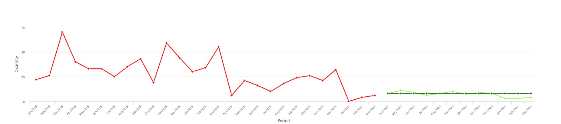
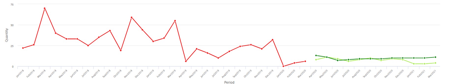
Each step in the data flow needs verification and validation.  Verification means the data at one step is still the same after flowing to the next step.  Validation means the data is correct and usable for analysis. 

The most common data flow looks like this:

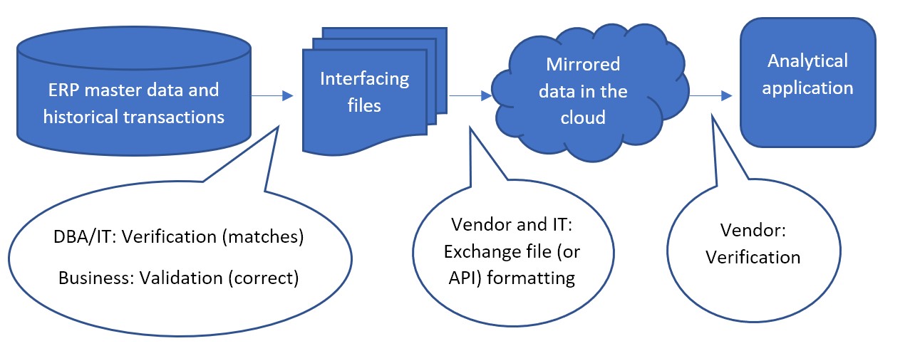
Less commonly, the first step between ERP master data and the interfacing files can sometimes be bypassed, where files are not used as an interface.  Instead, an API built by IT or the inventory optimization software vendor is responsible for data to be written directly from the ERP to the mirrored database in the cloud.  The vendor would work with IT to confirm the API is working as expected.  But the first validation step, even in that case, can still be performed.  After ingesting the data, the vendor can make the mirrored data available in files for the DBA/IT verification and business validation.

The confirmation that the mirrored data in the cloud completes the flow into the application is the responsibility of the vendor of software as a service.  SaaS vendors continually test that the software works correctly between the front-end application their subscribers see and the back-end data in the cloud database. If the subscribers still think the data doesn’t make sense in the application even after validating the interfacing files before going live, that is an issue to raise with the vendor’s customer support.

However the interfacing files are obtained, the largest part of verification and validation falls to the project manager and their team.  They must resource a test of the interfacing files to confirm:

1. They match the data in the ERP. And that all and only the ERP data that was necessary to extract for use in the application was extracted.
2. Nothing “jumps out” to the business as incorrect for each of the types of information in the data
3. They are formatted as expected.

DBA/IT Verification Tasks

1. Test the extract:

IT’s verification step can be done with various tools, comparing files, or importing files back to the database as temporary tables and joining them with the original data to confirm a match.  IT can depend on a query to pull the requested data into a file but that file can fail to match. The existence of delimiters or line returns within the data values can cause a file to be different than its original database table.  It is because the file relies heavily on delimiters and line returns to identify fields and records, while the table doesn’t rely on those characters to define its structure.

2. No bad characters:

Free form data entry fields in the ERP, such as product descriptions, can sometimes themselves contain line returns, tabs, commas, and/or double quotes that can affect the structure of the output file.  Line returns should not be allowed in values that will be extracted to a file.  Characters equal to the delimiter should be stripped during extract or else a different delimiter used.

Tip: if commas are the file delimiter, numbers greater than 999 can’t be extracted with a comma. Use “1000” rather than “1,000”.

3. Confirm the filters:

The other way that query extracts can return unexpected results is if conditions on the query are entered incorrectly.  The simplest way to avoid mistaken “where clauses” is to not use them.  Extract all data and allow the vendor to filter out some records according to rules supplied by the business.  If this will produce extract files so large that too much computing time is spent on the data exchange, the DBA/IT team should meet with the business to confirm exactly what filters on the data can be applied to avoid exchanging records that are meaningless to the application.

Tip: Bear in mind that Active/Inactive or item lifecycle information should not be used to filter out records.  This information should be sent to the application so it knows when an item becomes inactive.

4. Be consistent:

The extract process must produce files of consistent format every time it is executed.  File names, field names, and position, delimiter, and Excel sheet name if Excel is used, numeric formats and date formats, and the use of quotes around values should never differ from one execution of the extract one day to the next. A hands-off report or stored procedure should be prepared and used for every execution of the extract.

Business Validation Background

Below is a break down each of validation step into considerations, specifically in the case where the vendor has provided a template format for the interfacing files where each type of information is provided in its own file.  Files sent from your ERP to Smart are formatted for easy export from the ERP.  That sort of format makes the comparison back to the ERP a relatively simple job for IT, but it can be harder for the business to interpret.  Best practice is to manipulate the ERP data, either by using pivot tables or similar in a spreadsheet.  IT may assist by providing re-formatted data files for review by the business.

To delve into the interfacing files, you’ll need to understand them.  The vendor will supply a precise template, but generally interfacing files consist into three types: catalog data, item attributes, and transactional data.

• Catalog data contains identifiers and their attributes. Identifiers are typically for products, locations (which could be plants or warehouses), your customers, and your suppliers.
• Item attributes contain information about products at locations that are needed for analysis on the product and location combination. Such as:
  • Current replenishment policy in the form of a Min and Max, Reorder Point, or Review Period and Order Up To value, or Safety Stock
  • Primary supplier assignment and nominal lead time and cost per unit from that supplier
  • Order quantity requirements such as minimum order quantity, manufacturing lot size, or order multiples
  • Active/Inactive status of the product/location combination or flags that identify its state in its lifecycle, such as pre-obsolete
  • Attributes for grouping or filtering, such as assigned buyer/planner or product category
  • Current inventory information like on hand, on order, and in transit quantities.
• Transactional data contains references to identifiers along with dates and quantities. Such as quantity sold in a sales order of a product, at a location, for a customer, on a date.  Or quantity placed on purchase order of a product, into a location, from a supplier, on a date. Or quantity used in a work order of a component product at a location on a date.

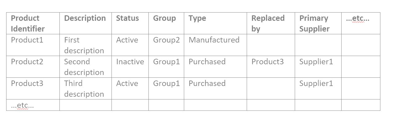
Validating Catalog Data

Considering catalog data first, you may have catalog files similar to these examples:

1: Check for a reasonable count of catalog records

For each file of catalog data, open it in a spreadsheet tool like Google Sheets or MS Excel. Answer these questions:

1. Is the record count in the ballpark? If you have about 50K products, there should not be only 10K rows in its file.
2. If it’s a short file, maybe the Location file, you can confirm exactly that all expected Iidentifiers are in it.
3. Filter by each attribute value and confirm again the count of records with that attribute value makes sense.

2: Check the correctness of values in each attribute field

Someone who knows what the products are and what the groups mean needs to take the time to confirm it is actually right, for all the attributes of all the catalog data.

So, if your Product file contains the attributes as in the example above, you would filter for Status of Active, and check that all resulting products are actually active.  Then filter for Status of Inactive and check that all resulting products are actually inactive.  Then filter for the first Group value and confirm all resulting products are in that group.  Repeat for Group2 and Group3, etc.  Then repeat for every attribute in every file.

It can help to do this validation with a comparison to an already existing and trusted report.  If you have another spreadsheet that shows products by Group for any reason, you can compare the interfacing files to it.  You may need to familiarize yourself with the VLOOKUP function that helps with spreadsheet comparison.

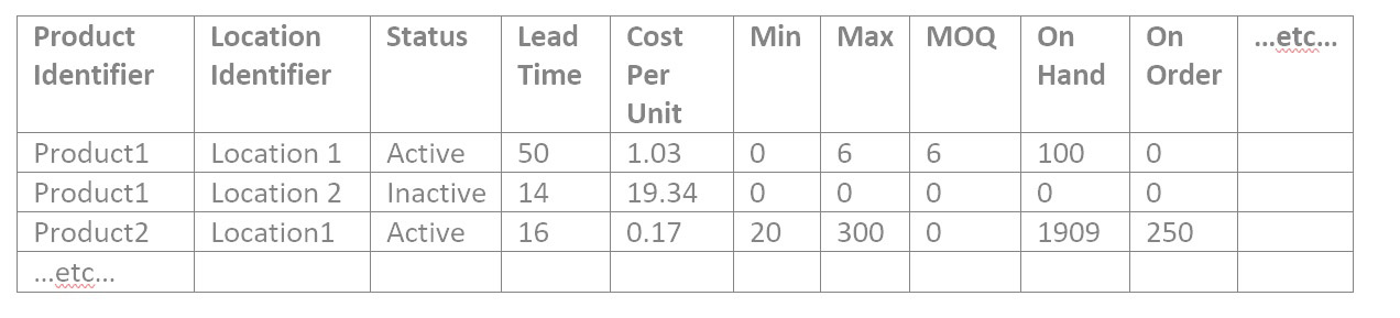
Validating Item Attribute Data

1: Check for a reasonable count of item records

The item attribute data confirmation is similar to the catalog data.  Confirm the product/location combination count makes sense in total and for each of the unique item attributes, one by one. This is an example item data file:

2: Find and explain weird numbers in item file

There tends to be many numerical values in the item attributes, so “weird” numbers merit review.  To validate data for a numerical attribute in any file, search for where the number is:

• Missing entirely
• Equal to zero
• Less than zero
• More than most others, or less than most others (sort by that column)
• Not a number at all, when it should be

A special consideration of files that are not catalog files is they may not show the descriptions of the products and locations, just their identifiers, which can be meaningless to you.  You can insert columns to hold the product and location descriptors that you are used to seeing and fill them into the spreadsheet to assist in your work.  The VLOOKUP function works for this as well.  Whether or not you have another report to compare the Items file to, you have the catalog files for Products and Location with show both the identifier and the description for each row.

3: Spot check

If you are frustrated to find that there are too many attribute values to manually check in a reasonable amount of time, spot checking is a solution. It can be done in a manner likely to pick up on any problems.  For each attribute, get a list of the unique values in each column.  You can copy a column into a new sheet, then use the Remove Duplicates function to see the list of possible values.   With it:

1. Confirm that no attribute values are present that shouldn’t be.
2. It can be harder to remember which attribute values are missing that should be there, so it can help to look at another source to remind you. For example, if Group1 through Group12 are present, you might check another source to remember if these are all the Groups possible.  Even if it is not required for the interfacing files for the application, it may be easy for IT to extract a list of all the possible Groups that are in your ERP which you can use for the validation exercise.  If you find extra or missing values that you don’t expect, bring an example of each to IT to investigate.
3. Sort alphabetically and scan down to see if any two values are similar but slightly different, maybe only in punctuation, which could mean one record had the attribute data entered incorrectly.

For each type of item, maybe one from each product group and/or location, check that all its attributes in every file are correct or at least pass a sanity check.  The more you can spot check from a broad range of items, the less likely you will have issues post go live.

Validating Transactional Data

Transactional files may all have a format similar to this:

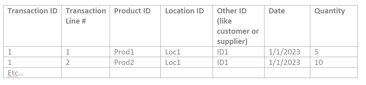
1: Find and explain weird numbers in each transactional file

These should be checked for “weird” numbers in the Quantity field.  Then you can proceed to:

1. Filter for dates outside the range you expect or missing expected dates entirely.
2. Find where Transaction identifiers and line numbers are missing. They shouldn’t be.
3. If there is more than one record for a given Transaction ID and Transaction Line Number combination, is that a mistake? Put another way, should duplicate records have their quantities summed together or is that double counting?

2: Sanity check summed quantities

Do a sanity check by filtering to a particular product you’re familiar with, and filter to a relatable date range such as last month or last year, and sum the quantities.  Is that total amount what you expected for that product in that time frame?  If you have information on total usage out of a location, you can slice the data that way to sum the quantities and compare to what you expect.  Pivot tables come in handy for verification of transactional data.  With them, you can view the data like:

The products’ yearly total may be simple to sanity check if you know the products well.  Or you can VLOOKUP to add attributes, such as product group, and pivot on that to see a higher level that is more familiar:

3: Sanity check count of records

It may help to display a count of transactions rather than a sum of the quantities, especially for purchase order data.  Such as:

And/or the same summarization at a higher level, like:

4: Spot checking

Spot checking the correctness of a single transaction, for each type of item and each type of transaction, completes due diligence.  Pay special attention to what date is tied to the transaction, and whether it is right for the analysis.  Dates may be a creation date, like the date a customer placed an order with you, or a promise date, like the date you expected to deliver on the customer’s order at the time of creating it, or a fulfilment date, when you actually delivered on the order.  Sometimes a promise date gets modified days after creating the order if it can’t be met.  Make sure the date in use reflects actual demand by the customer for the product most closely.

What to do about bad data 

If the mis-entries are few or one-off, you can edit the ERP records by hand as they are found, cleaning up your catalog attributes, even after go-live with the application.  But if large swathes of attributes or transaction quantities are off, this can spur an internal project to re-enter data correctly and possibly to change or start to document the process that needs to be followed when new records are entered into your ERP.

Care must be taken to avoid too long a delay in implementation of the SaaS application while waiting on clean attributes.  Break the work into chunks and use the application to analyze the clean data first so the data cleansing project occurs in parallel with getting value out of the new application.

Smart IP&O offers automated statistical forecasting that selects the right forecast method that best forecasts the data.  It does this for each time-series in the data set.  This blog will help a laymen understand how the forecast methods are chosen automatically.

Smart makes many methods available including single and double exponential smoothing, linear and simple moving average, and Winters models.  Each model is designed to capture a different sort of pattern.  The criteria to automatically choose one statistical method out of a set of choices is based on which method came closest to correctly predicting held-out history.

Earlier demand history is passed to each method and the result is compared to actuals to find the one that came closest overall.  That “winning” automatically chosen method is then fed all the history for that item to produce the forecast.

The overall nature of the demand pattern for the item is captured by holding out different portions of the history so that an occasional outlier does not unduly influence the choice of method.  You can visualize it using the below diagram where each row represents a 3-period forecast in held out history, based on different amounts of the red earlier history.  The variances of each pass are averaged together to determine the method’s overall ranking against all other methods.

For most time series, this process can accurately capture trends, seasonality, and average volume accurately. But sometimes a chosen method comes mathematically closest to predicting the held-out history but doesn’t project it forward in a way that makes sense.

Users can correct this by using the system’s exception reports and filtering features to identify items that merit review.  They can then configure the automatic forecast methods that they wish to be considered for that item.