Lead time delays and supply variability are supply chain facts of life, yet inventory-carrying organizations are often caught by surprise when a supplier is late. An effective inventory planning process embraces this fact of life and develops policies that effectively account for this uncertainty. Sure, there will be times when lead time delays come out of nowhere and cause a shortage. But most often, the shortages result from:

1. Not computing stocking policies (e.g., reorder points, safety stocks, and Min/Max levels) often enough to catch changes in the lead time. 
2. Using poor estimates of actual lead time such as using only averages of historical receipts or relying on a supplier quote.

Instead, recalibrate policies across every single part during every planning cycle to catch changes in demand and lead times.  Rather than assuming only an average lead time, simulate the lead times using scenarios.  This way, recommended stocking policies account for the probabilities of lead times being high and adjust accordingly.  When you do this, you’ll identify needed inventory increases before it is too late. You’ll capture more sales and drive significant improvements in customer satisfaction.

Summary

Smart Software’s advanced supply chain analytics exploits multiple advanced methods. Two of the most important are “statistical bootstrapping” and “Monte Carlo simulation”. Since both involve lots of random numbers flying around, folks sometimes get confused about which is which and what they are good for. Hence, this note. Bottom line up front: Statistical bootstrapping generates demand scenarios for forecasting. Monte Carlo simulation uses the scenarios for inventory optimization.

Bootstrapping

Bootstrapping, also called “resampling” is a method of computational statistics that we use to create demand scenarios for forecasting. The essence of the forecasting problem is to expose possible futures that your company might confront so you can work out how to manage business risks. Traditional forecasting methods focus on computing “most likely” futures, but they fall short of presenting the full risk picture. Bootstrapping provides an unlimited number of realistic what-if scenarios.

Bootstrapping does this without making unrealistic assumptions about the demand, i.e., that it is not intermittent, or that it has a bell-shaped distribution of sizes. Those assumptions are crutches to make the math simpler, but the bootstrap is a procedure,  not an equation, so it doesn’t need such simplifications.

For the simplest demand type, which is a stable randomness with no seasonality or trend, bootstrapping is dead easy. To get a reasonable idea of what a single future demand value might be, pick one of the historical demands at random. To create a demand scenario, make multiple random selections from the past and string them together. Done. It is possible to add a little more realism by “jittering” the demand values, i.e., adding or subtracting a bit of additional randomness to each one, but even that is simple.

Figure 1 shows a simple bootstrap. The first line is a short sequence of historical demand for an SKU. The following lines show scenarios of future demand created by randomly selecting values from the demand history. For instance, the next three demand might be (0, 14, 6), or (2, 3, 5), etc.

Figure 1: Example of demand scenarios generated by a simple bootstrap

Higher frequency operations such as daily forecasting bring with them more complex demand patterns, such as double seasonality (e.g., day-of-week and month-of-year) and/or trend. This challenged us to invent a new generation of bootstrapping algorithms. We recently won a US Patent for this breakthrough, but the essence is as described above.

Monte Carlo Simulation

Monte Carlo is famous for its casinos, which, like bootstrapping, invoke the idea of randomness. Monte Carlo methods go back a long way, but the modern impetus came with the need to do some hairy calculations about where neutrons would fly when an A-bomb explodes.

The essence of Monte Carlo analysis is this: “Our problem is too complicated to analyze with paper-and-pencil equations. So, let’s write a computer program that codes the individual steps of the process, put in the random elements (e.g., which way a neutron shoots away), wind it up and watch it go. Since there’s a lot of randomness, let’s run the program a zillion times and average the results.”

Applying this approach to inventory management, we have a different set of randomly occurring events: e.g., a demand of a given size arrives on a random day, a replenishment of a given size arrives after a random lead time, we cut a replenishment PO of a given size when stock drops to or below a given reorder point. We code the logic relating these events into a program. We feed it with a random demand sequence (see bootstrapping above), run the program for a while, say one year of daily operations, compute performance metrics like Fill Rate and Average On Hand inventory, and “toss the dice” by re-running the program many times and averaging the results of many simulated years. The result is a good estimate of what happens when we make key management decisions: “If we set the reorder point at 10 units and the order quantity at 15 units, we can expect to get a service level of 89% and an average on hand of 21 units.” What the simulation is doing for us is exposing the consequences of management decisions based on realistic demand scenarios and solid math. The guesswork is gone.

Figure 2 shows some of the inner workings of a Monte Carlo simulation of an inventory system in four panels. The system uses a Min/Max inventory control policy with Min=10 and Max=25. No backorders are allowed: you have the good or you lose the business. Replenishment lead times are usually 7 days but sometimes 14. This simulation ran for one year.

The first panel shows a complex random demand scenario in which there is no demand on weekends, but demand generally increases each day from Monday to Friday. The second panel shows the random number of units on hand, which ebbs and flows with each replenishment cycle. The third panel shows the random sizes and timings of replenishment orders coming in from the supplier. The final panel shows the unsatisfied demand that jeopardizes customer relationships. This kind of detail can be very useful for building insight into the dynamics of an inventory system.

Figure 2: Details of a Monte Carlo simulation

Figure 2 shows only one of the countless ways that the year could play out. Generally, we want to average the results of many simulated years. After all, nobody would flip a coin once to decide if it were a fair coin. Figure 3 shows how four key performance metrics (KPI’s) vary from year to year for this system. Some metrics are relatively stable across simulations (Fill Rate), but others show more relative variability (Operating Cost= Holding Cost + Ordering Cost + Shortage Cost). Eyeballing the plots, we can estimate that the choices of Min=10, Max=25 leads to an average Operating cost of around $3,000 per year, a Fill Rate of around 90%, a Service Level of around 75%, and an Average On Hand of about 10

Figure 3: Variation in KPI’s computed over 1,000 simulated years

In fact, it is now possible to answer a higher level of management question. We can go beyond “What will happen if I do such-and-such?” to “What is the best thing I can do to achieve a fill rate of at least 90% for this item at the lowest possible cost?” The mathemagic  behind this leap is yet another key technology called “stochastic optimization”, but we’ll stop here for now. Suffice it to say that Smart’s SIO&P software can search the “design space” of Min and Max values to automatically find the best choice.

Is safety stock regarded as emergency spares or as a day-to-day buffer against spikes in demand? Knowing the difference and configuring your ERP properly will make a big difference to your bottom line.

The Safety Stock field in your ERP system can mean very different things depending on the configuration. Not understanding these differences and how they impact your bottom line is a common issue we’ve seen arise in implementations of our software.

Implementing inventory optimization software starts with new customers completing the technical implementation to get data flowing.  They then receive user training and spend weeks carefully configuring their initial safety stocks, reorder levels, and consensus demand forecasts with Smart IP&O.  The team becomes comfortable with Smart’s key performance predictions (KPPs) for service levels, ordering costs, and inventory on hand, all of which are forecasted using the new stocking policies.

But when they save the policies and forecasts to their ERP test system, sometimes the orders being suggested are far larger and more frequent than they expected, driving up projected inventory costs.

When this happens, the primary culprit is how the ERP is configured to treat safety stock.  Being aware of these configuration settings will help planning teams better set expectations and achieve the expected outcomes with less effort (and cause for alarm!).

Here are the three common examples of ERP safety stock configurations:

Configuration 1. Safety Stock is treated as emergency stock that can’t be consumed. If a breach of safety stock is predicted, the ERP system will force an expedite no matter the cost so the inventory on hand never falls below safety stock, even if a scheduled receipt is already on order and scheduled to arrive soon.

Configuration 2. Safety Stock is treated as Buffer stock that is designed to be consumed. The ERP system will place an order when a breach of safety stock is predicted but on hand inventory will be allowed to fall below the safety stock. The buffer stock protects against stockout during the resupply period (i.e., the lead time).

Configuration 3. Safety Stock is ignored by the system and treated as a visual planning aid or rule of thumb. It is ignored by supply planning calculations but used by the planner to help make manual assessments of when to order.

Note: We never recommend using the safety stock field as described in Configuration 3. In most cases, these configurations were not intended but result from years of improvisation that have led to using the ERP in a non-standard way.  Generally, these fields were designed to programmatically influence the replenishment calculations.  So, the focus of our conversation will be on Configurations 1 and 2. 

Forecasting and inventory optimization systems are designed to compute forecasts that will anticipate inventory draw down and then calculate safety stocks sufficient to protect against variability in demand and supply. This means that the safety stock is intended to be used as a protective buffer (Configuration 2) and not as emergency sparse (Configuration 3).  It is also important to understand that, by design, the safety stock will be consumed approximately 50% of the time.

Why 50%? Because actual orders will exceed an unbiased forecast half of the time. See the graphic below illustrating this.  A “good” forecast should yield the value that will come closest to the actual most often so actual demand will either be higher or lower without bias in either direction.

If you configured your ERP system to properly allow consumption of safety stock, then the on hand inventory might look like the graph below.  Note that some safety stock is consumed but avoided a stockout.  The service level you target when computing safety stock will dictate how often you stockout before the replenishment order arrives.  Average inventory is roughly 60 units over the time horizon in this scenario.

If your ERP system is configured to not allow consumption of safety stock and treats the quantity entered in the safety stock field more like emergency spares, then you will have a massive overstock!  Your inventory on hand would look like the graph below with orders being expedited as soon as a breach of safety stock is expected. Average inventory is roughly 90 units, a 50% increase compared to when you allowed safety stock to be consumed.

Managing spare parts presents numerous challenges, such as unexpected breakdowns, changing schedules, and inconsistent demand patterns. Traditional forecasting methods and manual approaches are ineffective in dealing with these complexities. To overcome these challenges, this blog outlines key strategies that prioritize service levels, utilize probabilistic methods to calculate reorder points, regularly adjust stocking policies, and implement a dedicated planning process to avoid excessive inventory. Explore these strategies to optimize spare parts inventory and improve operational efficiency.

Bottom Line Upfront

​1.Inventory Management is Risk Management.

2.Can’t manage risk well or at scale with subjective planning – Need to know service vs. cost.

3.It’s not supply & demand variability that are the problem – it’s how you handle it.

4.Spare parts have intermittent demand so traditional methods don’t work.

5.Rule of thumb approaches don’t account for demand variability and misallocate stock.

6.Use Service Level Driven Planning  (service vs. cost tradeoffs) to drive stock decisions.

7.Probabilistic approaches such as bootstrapping yield accurate estimates of reorder points.

8.Classify parts and assign service level targets by class.

9.Recalibrate often – thousands of parts have old, stale reorder points.

10.Repairable parts require special treatment.

Do Focus on the Real Root Causes

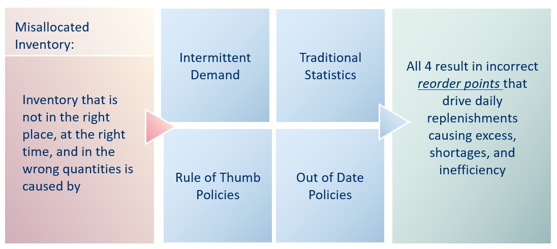
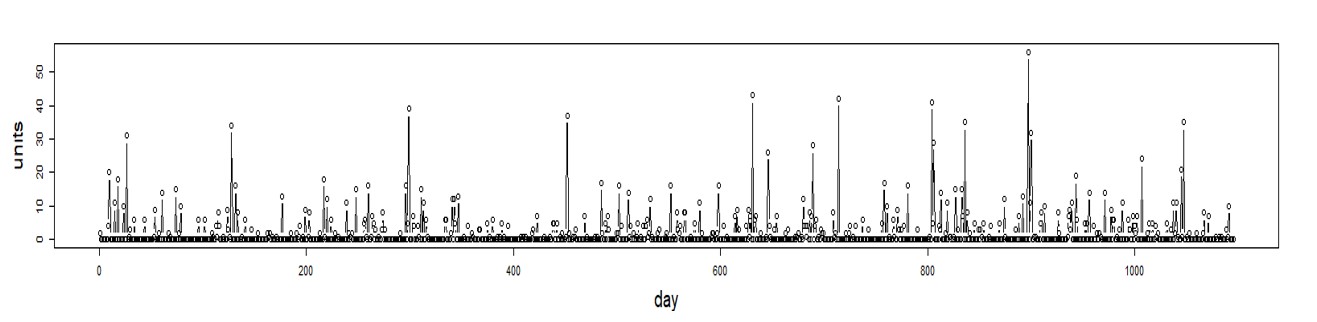
Intermittent Demand

• Slow moving, irregular or sporadic with a large percentage of zero values.
• Non-zero values are mixed in randomly – spikes are large and varied.
• Isn’t bell shaped (demand is not Normally distributed around the average.)
• At least 70% of a typical Utility’s parts are intermittently demanded.

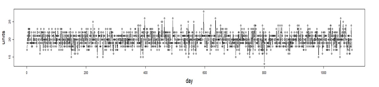
Normal Demand

• Very few periods of zero demand (exception is seasonal parts.)
• Often exhibits trend, seasonal, or cyclical patterns.
• Lower levels of demand variability.
• Is bell-shaped (demand is Normally distributed around the average.)

Don’t rely on averages

• OK for determining typical usage over longer periods of time.
• Often forecasts more “accurately” than some advanced methods.
• But…insufficient for determining what to stock.

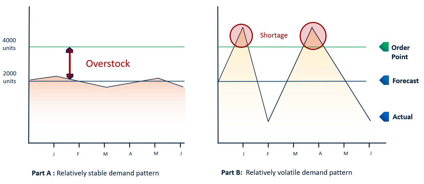
Don’t Buffer with Multiples of Averages

Example:  Two equally important parts so let’s treat them the same.
We’ll order more  when On Hand Inventory ≤ 2 x Avg Lead Time Demand.

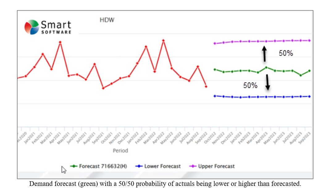
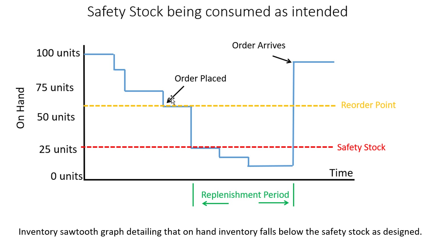
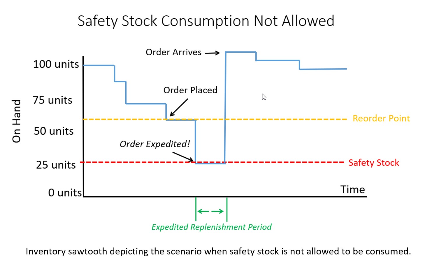
Do use Service Level tradeoff curves to compute safety stock

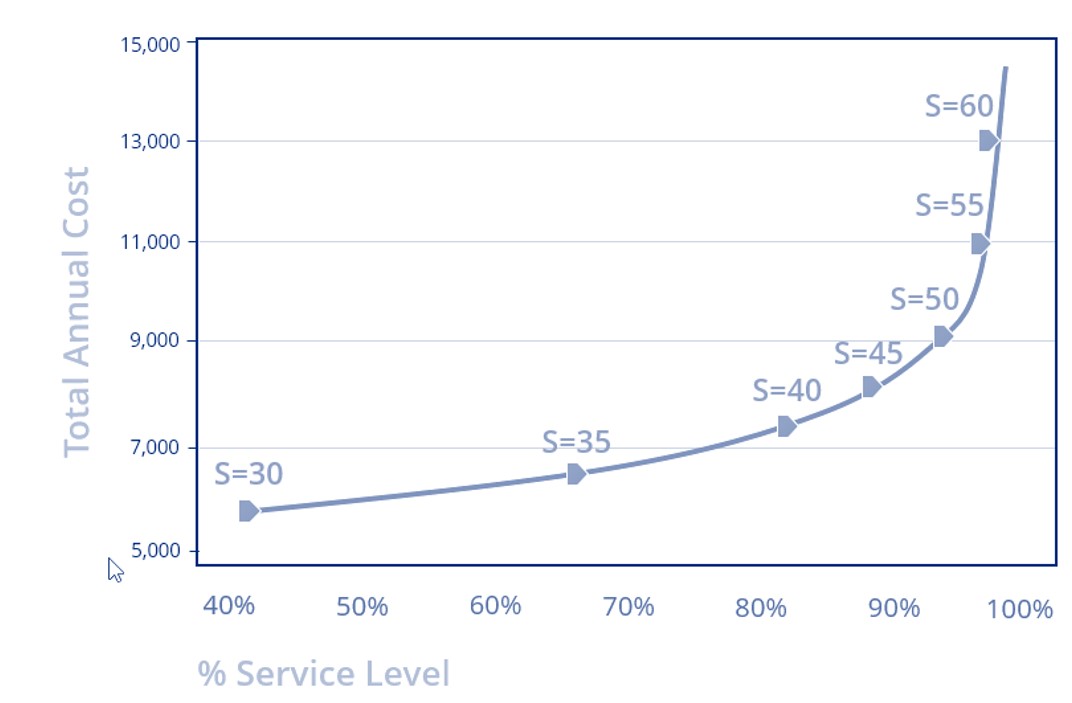
Standard Normal Probabilities

OK for normal demand. Doesn’t work with intermittent demand!

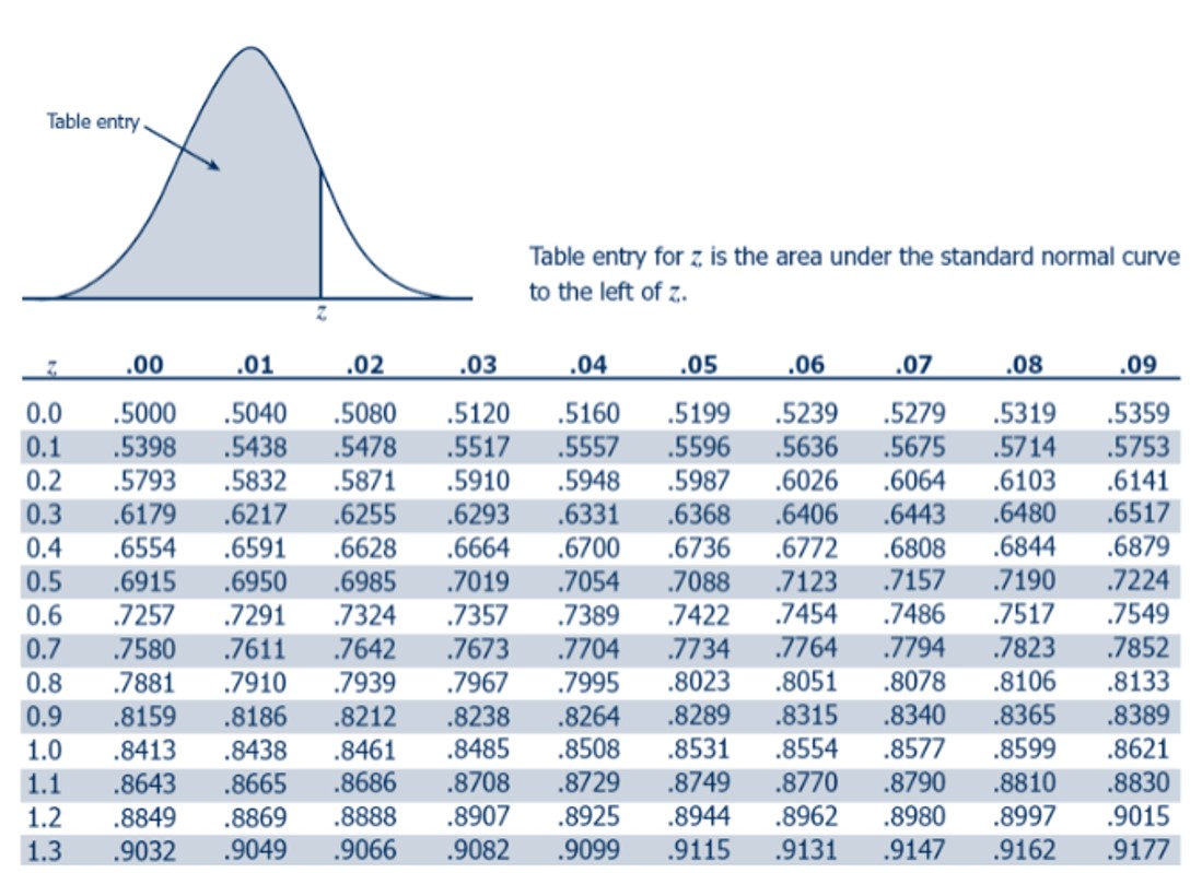
Don’t use Normal (Bell Shaped) Distributions

• You’ll get the tradeoff curve wrong:

– e.g., You’ll target 95% but achieve 85%.

– e.g., You’ll target 99% but achieve 91%.

• This is a huge miss with costly implications:

– You’ll stock out more often than expected.

– You’ll start to add subjective buffers to compensate and then overstock.

– Lack of trust/second-guessing of outputs paralyzes planning.

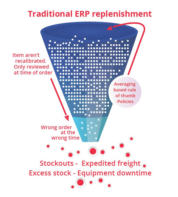
Why Traditional Methods Fail on Intermittent Demand: 

Traditional Methods are not designed to address core issues in spare parts management.

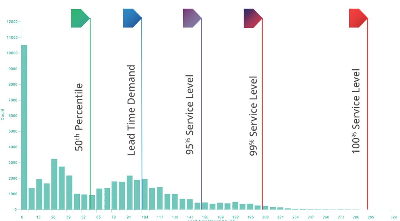
Need: Probability distribution (not bell-shaped) of demand over variable lead time.

• Get: Prediction of average demand in each month, not a total over lead time.
• Get: Bolted-on model of variability, usually the Normal model, usually wrong.

Need: Exposure of tradeoffs between item availability and cost of inventory.

• Get: None of this; instead, get a lot of inconsistent, ad-hoc decisions.

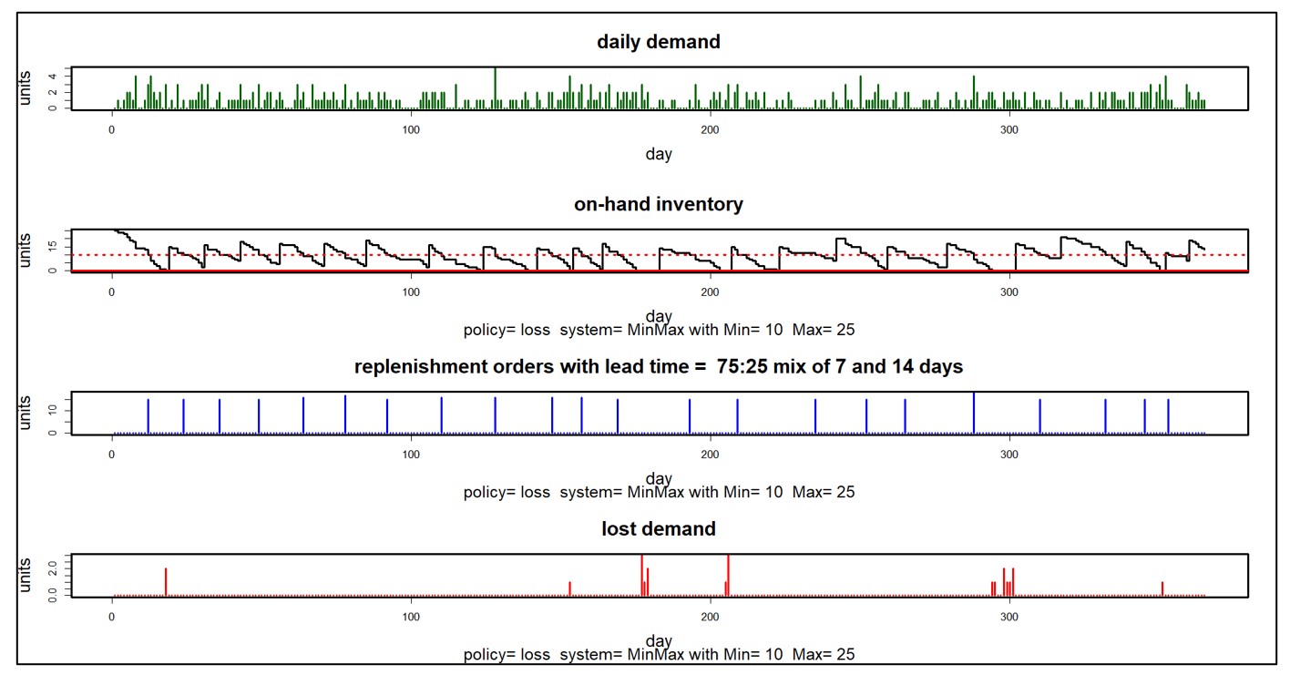
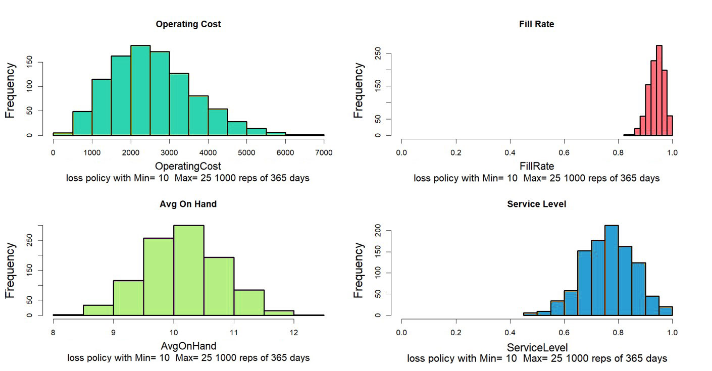
Do use Statistical Bootstrapping to Predict the Distribution:

Then exploit the distribution to optimize stocking policies.

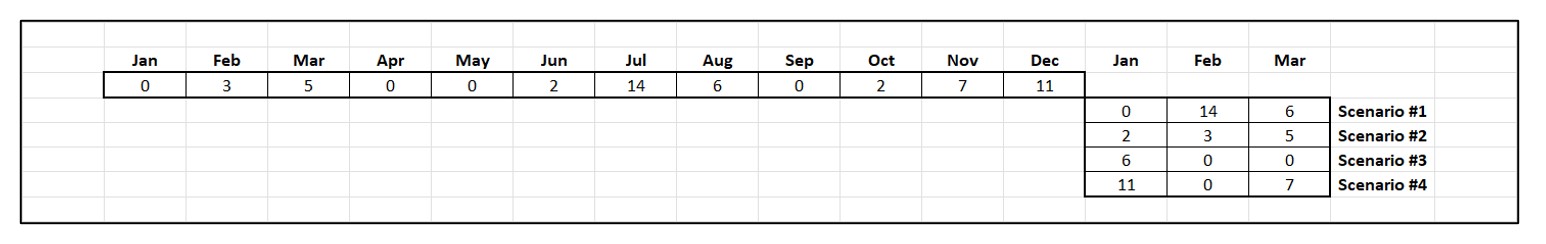
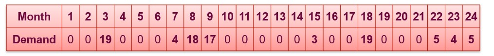
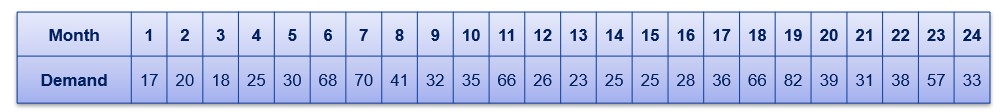
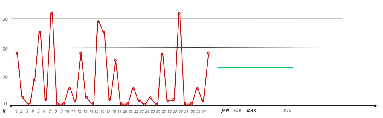
How does Bootstrapping Work?

24 Months of Historical Demand Data.

Bootstrap Scenarios for a 3-month Lead Time.

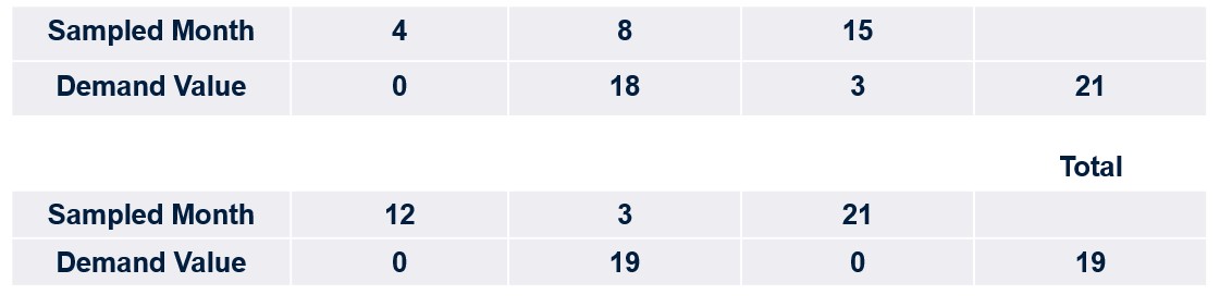
Bootstrapping Hits the Service Level Target with nearly 100% Accuracy!

• National Warehousing Operation.

Task: Forecast inventory stocking levels for 12,000 intermittently demanded SKUs at 95% & 99% service levels

Results:

At 95% service level, 95.23% did not stock out.

At 99% service level, 98.66% did not stock out.

This means you can rely on output to set expectations and confidently make targeted stock adjustments that lower inventory and increase service.

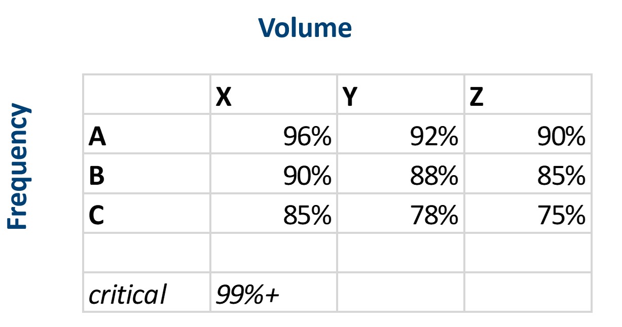
Set Target Service Levels According to Order Frequency & Size

Recalibrate Reorder Points Frequently

• Static ROPs cause excess and shortages.
• As lead time increases, so should the ROP and vice versa.
• As usage decreases, so should the ROP and vice versa.
• Longer you wait to recalibrate, the greater the imbalance.
• Mountains of parts ordered too soon or too late.
• Wastes buyers’ time placing the wrong orders.
• Breeds distrust in systems and forces data silos.

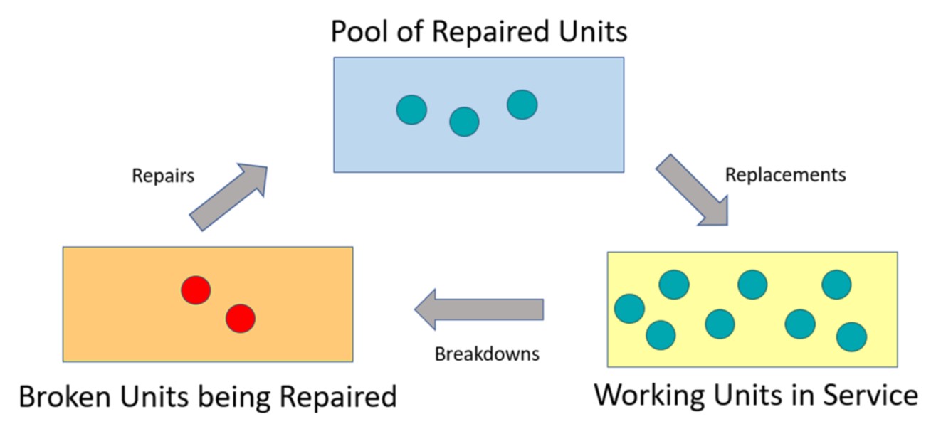
Do Plan Rotables (Repair Parts) Differently

Summary

1.Inventory Management is Risk Management.

2.Can’t manage risk well or at scale with subjective planning – Need to know service vs. cost.

3.It’s not supply & demand variability that are the problem – it’s how you handle it.

4.Spare parts have intermittent demand so traditional methods don’t work.

5.Rule of thumb approaches don’t account demand variability and misallocate stock.

6.Use Service Level Driven Planning  (service vs. cost tradeoffs) to drive stock decisions.

7.Probabilistic approaches such as bootstrapping yield accurate estimates of reorder points.

8.Classify parts and assign service level targets by class.

9.Recalibrate often – thousands of parts have old, stale reorder points.

10.Repairable parts require special treatment.

We often are asked, “Why is the software driving up the inventory?” The answer is that Smart isn’t driving it in either direction – the inputs are driving it, and those inputs are controlled by the users (or admins). Here are four things you can do to get the results you expect.

1. Confirm that your service level targets are commensurate with what you want for that item or group of items. Setting very high targets (95% or more) will likely drive inventory up if you have been coasting along at a lower level and are OK with being there. It’s possible you’ve never achieved the new higher service level but customers have not complained.  Figure out what service level has worked by evaluating historical reports on performance and set your targets accordingly. But keep in mind that competitors may beat you on item availability if you keep using your father’s service level targets.

2. Make sure your understanding of “service level” aligns with the software system’s definition. You may be measuring performance based on how often you ship within one week from receipt of the customer order, whereas the software is targeting reorder points based on your ability to ship right away, not within a week. Clearly the latter will require more inventory to hit the same “service level.” For instance, a 75% same-day service level may correspond to a 90% same-week service level. In this case, you are really comparing apples to oranges. If this is the reason for the excess stock, then determine what “same day” service level is needed to get you to your desired “same week” service level and enter that into the software. Using the less-stringent same-day target will drop the inventory, sometimes very significantly.

3. Evaluate the lead time inputs. We’ve seen instances in which lead times had been inflated to trick old software into producing desired results. Modern software tracks suppliers’ performance by recording their actual lead times over multiple orders, then it takes account of lead time variability in its simulations of daily operations. Watch out if your lead times are fixed at one value that was decided on in the distant past and isn’t current.

4. Check your demand signal. You have lots of historical transactions in your ERP system that can be used in many ways to determine the demand history. If you are using signals such as transfers, or you are not excluding returns, then you may be overstating demand. Spend a little time on defining “demand” in the way that makes most sense for your situation.