I’ve stood in front of thousands of students. They’ve been more or less young, more or less technical, more or less experienced – and more or less interested.  I’ve done this as a university faculty member since 1972, first at Massachusetts Institute of Technology, then at Harvard University, finally in the School of Engineering at Rensselaer Polytechnic Institute. Between Harvard and RPI I dropped out of academia temporarily to co-found Smart Software with Charlie Smart and Nelson Hartunian. So since then, I’ve also been busy training business users to exploit the power of advanced analytics for forecasting and inventory optimization.

As I write this, I’ve just returned to my office at RPI after introducing first-year Industrial Engineering students to the basic concepts of inventory management. If they stick with the program, they will go on to take required courses in supply chain, system simulation, statistical analysis, and optimization. I told them stories about how useful they will be to their companies should they decide to make a career in the world of supply chain. If I’d had more time, I would have mentioned how capable they will be when they graduate relative to many of their corporate peers. These freshmen and ready and willing to stay the course, soaking up all the techniques and theories we can throw at them, and honing their practical skills in summer jobs or coop assignments.

What I didn’t tell them is that many of them will have to work to keep their intensity when they are on the job. It’s a sad truth that, for whatever reason, many inventory practitioners settle into a kind of stasis that impedes their companies’ ability to exploit the latest technologies, such as cloud-based advanced demand forecasting and inventory optimization. Gather enough of such people in one place and agility and improved efficiency go out the window.

I think one of the factors that dulls people is that the process of implementation frequently feels painfully incremental and prolonged. It often begins with a sobering inventory of relevant data, its correctness, and its currency. Then it moves to an often-awkward discovery that there really is no systematic process in place and the subsequent need to design a good one going forward. Next is the need to learn to use a new software suite. That step involves learning new vocabulary, some level of probabilistic thought, an ability to interpret new graphs and tables, not to mention a new software interface.  All this takes time and effort.

We’ve found that a few things help new customers stay the course. One is having a champion among management, an executive sponsor, who can vouch for the commercial importance of a successful implementation while ensuring the users are supported with continuing education.  A second is identifying and training a super-user or two having unusual combinations of technical and communication skills.  A third is breaking the training into bite-sized chunks and testing for comprehension after each chunk and repeating this process until it is clear that the new concepts, vocabulary, and process are fully absorbed. But all those maneuvers will come to naught without management being all-in and ready to stay the course.  Inventory planning practices in place for many years are not going to be replaced entirely over a three-month implementation process.  You’ve got to want it to get it.

Managing the inventory in a single facility is difficult enough, but the problem becomes much more complex when there are multiple facilities arrayed in multiple echelons. The complexity arises from the interactions among the echelons, with demands at the lower levels bubbling up and any shortages at the higher levels cascading down.

If each of the facilities were to be managed in isolation, standard methods could be used, without regard to interactions, to set inventory control parameters such as reorder points and order quantities. However, ignoring the interactions between levels can lead to catastrophic failures. Experience and trial and error allow the design of stable systems, but that stability can be shattered by changes in demand patterns or lead times or by the addition of new facilities. Coping with such changes is greatly aided by advanced supply chain analytics, which provide a safe “sandbox” within which to test out proposed system changes before deploying them. This blog illustrates that point.

The Scenario

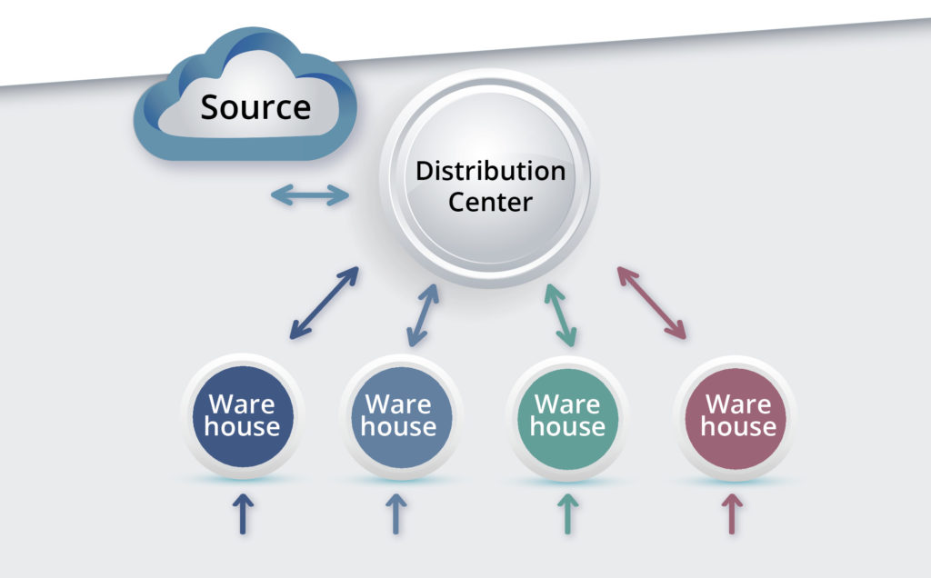
To have some hope of discussing this problem usefully, this blog will simplify the problem by considering the two-level hierarchy pictured in Figure 1. Imagine the facilities at the lower level to be warehouses (WHs) from which customer demands are meant to be satisfied, and that the inventory items at each WH are service parts sold to a wide range of external customers.

Figure 1: General structure of one type of two-level inventory system

Imagine the higher level to consist of a single distribution center (DC) which does not service customers directly but does replenish the WHs. For simplicity, assume the DC itself is replenished from a Source that always has (or makes) sufficient stock to immediately ship parts to the DC, though with some delay. (Alternatively, we could consider the system to have retail stores supplied by one warehouse).

Each level can be described in terms of demand levels (treated as random), lead times (random), inventory control parameters (here, Min and Max values) and shortage policy (here, backorders allowed).

The Method of Analysis

The academic literature has made progress on this problem, though usually at the cost of simplifications necessary to facilitate a purely mathematical solution. Our approach here is more accessible and flexible: Monte Carlo simulation. That is, we build a computer program that incorporates the logic of the system operation. The program “creates” random demand at the WH level, processes the demand according to the logic of a chosen inventory policy, and creates demand for the DC by pooling the random requests for replenishment made by the WHs. This approach lets us observe many simulated days of system operation while watching for significant events like stockouts at either level.

An Example

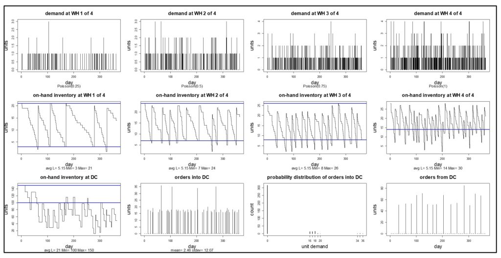
To illustrate an analysis, we simulated a system consisting of four WHs and one DC. Average demand varied across the WHs. Replenishment from the DC to any WH took from 4 to 7 days, averaging 5.15 days. Replenishment of the DC from the Source took either 7, 14, 21 or 28 days, but 90% of the time it was either 21 or 28 days, making the average 21 days. Each facility had Min and Max values set by analyst judgement after some rough calculations.

Figure 2 shows the results of one year of simulated daily operation of this system. The first row in the figure shows the daily demand for the item at each WH, which was assumed to be “purely random”, meaning it had a Poisson distribution. The second row shows the on-hand inventory at the end of each day, with Min and Max values indicated by blue lines. The third row describes operations at the DC.  Contrary to the assumption of much theory, the demand into the DC was not close to being Poisson, nor was the demand out of the DC to the Source. In this scenario, Min and Max values were sufficient to keep item availability was high at each WH and at the DC, with no stockouts observed at any of the five facilities.

Click here to enlarge the image

Figure 2 – Simulated year of operation of a system with four WHs and one DC.

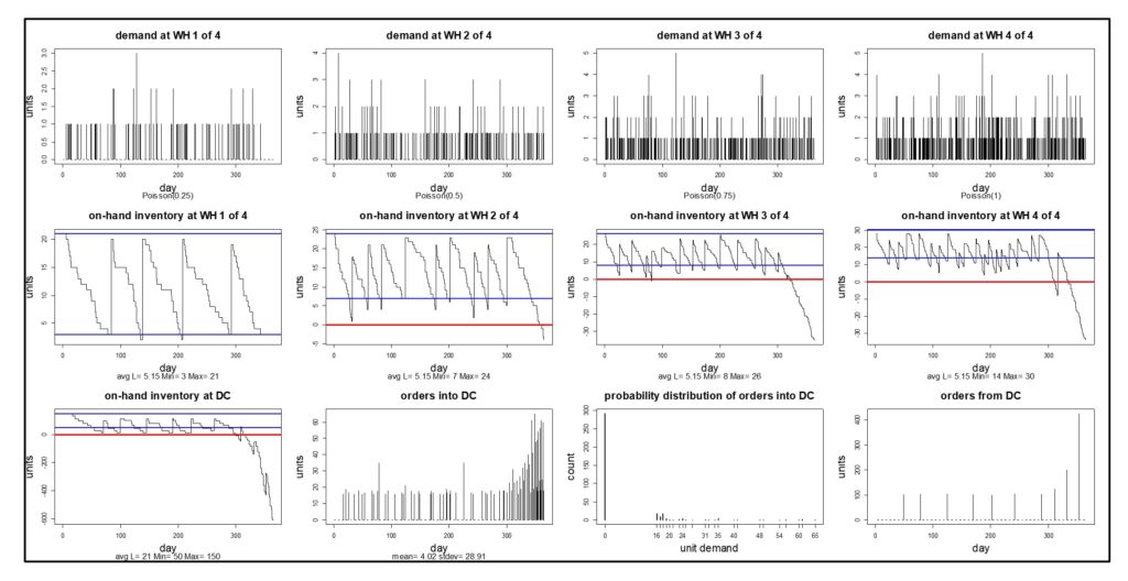
Now let’s vary the scenario. When stockouts are extremely rare, as in Figure 2, there is often excess inventory in the system. Suppose somebody suggests that the inventory level at the DC looks a bit fat and thinks it would be good idea to save money there. Their suggestion for reducing the stock at the DC is to reduce the value of the Min at the DC from 100 to 50. What happens? You could guess, or you could simulate.

Figure 3 shows the simulation – the result is not pretty. The system runs fine for much of the year, then the DC runs out of stock and cannot catch up despite sending successively larger replenishment orders to the Source. Three of the four WHs descend into death spirals by the end of the year (and WH1 follows thereafter). The simulation has highlighted a sensitivity that cannot be ignored and has flagged a bad decision.

Click here to enlarge image

Figure 3 – Simulated effects of reducing the Min at the DC.

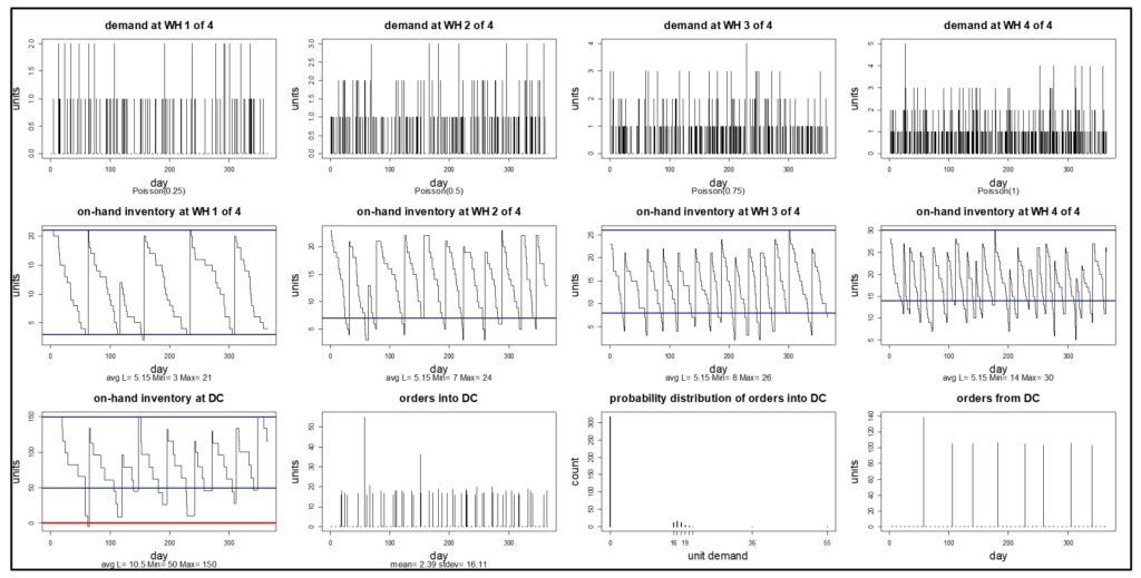
Now the inventory managers can go back to the drawing board and test out other possible ways to reduce the investment in inventory at the DC level. One move that always helps, if you and your supplier can jointly make it happen, is to create a more agile system by reducing replenishment lead time. Working with the Source to insure that the DC always gets its replenishments in either 7 or 14 days stabilizes the system, as shown in Figure 4.

Click here to enlarge image

Figure 4 – Simulated effects of reducing the lead time for replenishing the DC.

Unfortunately, the intent of reducing the inventory at the DC has not been achieved. The original daily inventory count was about 80 units and remains about 80 units after reducing the DC’s Min and drastically improving the Source-to-DC lead time. But with the simulation model, the planning team can try out other ideas until they arrive at a satisfactory redesign. Or, given that Figure 4 shows the DC inventory starting to flirt with zero, they might think it prudent to accept the need for an average of about 80 units at the DC and look for ways to trim inventory investment at the WHs instead.

The Takeaways

1. Multiechelon inventory optimization (MEIO) is complex. Many factors interact to produce system behaviors that can be surprising in even simple two-level systems.
2. Monte Carlo simulation is a useful tool for planners who need to design new systems or tweak existing systems.

For most small-to-medium manufacturers and distributors, single-level or single-echelon inventory optimization is at the cutting edge of logistics practice. Multi-echelon inventory optimization (“MEIO”) involves playing the game at an even higher level and is therefore much less common. This blog is the first of two. It aims to explain what MEIO is, why standard MEIO theories break down, and how probabilistic modeling through scenario simulation can restore reality to the MEIO process. The second blog will show a particular example.

Definition of Inventory Optimization

An inventory system is built on a set of design choices.

The first choice is the policy for responding to stockouts: Do you just lose the sale to a competitor, or can you convince the customer to accept a backorder? The former is more common with distributors than manufacturers, but this may not be much of a choice since customers may dictate the answer.

The second choice is the inventory policy. These divide into “continuous review” and “periodic review” policies, with several options within each type. You can link to a video tutorial describing several common inventory policies here.  Perhaps the most efficient is known to practitioners as “Min/Max” and to academics as (s, S) or “little S, Big S.” We use this policy in the scenario simulations below. It works as follows: When on-hand inventory drops to or below the Min (s), an order is placed for replenishment. The size of the order is the gap between the on-hand inventory and the Max (S), so if Min is 10, Max is 25 and on-hand is 8, it’s time for an order of 25-8 = 17 units.

The third choice is to decide on the best values of the inventory policy “parameters”, e.g., the values to use for Min and Max. Before assigning numbers to Min and Max, you need clarity on what “best” means for you. Commonly, best means choices that minimize inventory operating costs subject to a floor on item availability, expressed either as Service Level or Fill Rate. In mathematical terms, this is a “two-dimensional constrained integer optimization problem”. “Two-dimensional” because you have to pick two numbers: Min and Max. “Integer” because Min and Max have to be whole numbers. “Constrained” because you must pick Min and Max values that give a high-enough level of item availability such as service levels and fill rates. “Optimization” because you  want to get there with the lowest operating cost (operating cost combines holding, ordering and shortage costs).

Multiechelon Inventory Systems

The optimization problem becomes more difficult in multi-echelon systems. In a single-echelon system, each inventory item can be analyzed in isolation: one pair of Min/Max values per SKU. Because there are more parts to a multiechelon system, there is a bigger computational problem.

Figure 1 shows a simple two-level system for managing a single SKU. At the lower level, demands arrive at multiple warehouses. When those are in danger of stocking out, they are resupplied from a distribution center (DC). When the DC itself is in danger of stocking out, it is supplied by some outside source, such as the manufacturer of the item.

The design problem here is multidimensional: We need Min and Max values for 4 warehouses and for the DC, so the optimization occurs in 4×2+1×2=10 dimensions. The analysis must take account of a multitude of contextual factors:

• The average level and volatility of demand coming into each warehouse.
• The average and variability of replenishment lead times from the DC.
• The average and variability of replenishment lead times from the source.
• The required minimum service level at the warehouses.
• The required minimum service level at the DC.
• The holding, ordering and shortage costs at each warehouse.
• The holding, ordering and shortage costs at the DC.

As you might expect, seat-of-the-pants guesses won’t do well in this situation. Neither will trying to simplify the problem by analyzing each echelon separately. For instance, stockouts at the DC increase the risk of stockouts at the warehouse level and vice versa.

This problem is obviously too complicated to try to solve without help from some sort of computer model.

Why Standard Inventory Theory is Bad Math

With a little looking, you can find models, journal articles and book about MEIO. These are valuable sources of information and insight, even numbers. But most of them rely on the expedient of over-simplifying the problem to make it possible to write and solve equations. This is the “Fantasy” referred to in the title.

Doing so is a classic modeling maneuver and is not necessarily a bad idea. When I was a graduate student at MIT, I was taught the value of having two models: a small, rough model to serve as a kind of sighting scope and a larger, more accurate model to produce reliable numbers. The smaller model is equation-based and theory-based; the bigger model is procedure-based and data-based, i.e., a detailed system simulation. Models based on simple theories and equations can produce bad numerical estimates and even miss whole phenomena. In contrast, models based on procedures (e.g., “order up to the Max when you breach the Min”) and facts (e.g., the last 3 years of daily item demand) will require a lot more computing but give more realistic answers. Luckily, thanks to the cloud, we have a lot of computing power at our fingertips.

Perhaps the greatest modeling “sin” in the MEIO literature is the assumption that demands at all echelons can be modeled as purely random Poisson processes. Even if it were true at the warehouse level, it would be far from true at the DC level. The Poisson process is the “white rat of demand modeling” because it is simple and permits more paper-and-pencil equation manipulation. Since not all demands are Poisson shaped, this results in unrealistic recommendations.

Scenario-based Simulation Optimization

To get realism, we must get down into the details of how the inventory systems operate at each echelon. With few limits except those imposed by hardware such as size of memory, computer programs can keep up any level of complexity. For instance, there is no need to assume that each of the warehouses faces identical demand streams or has the same costs as all the others.

A computer simulation works as follows.

1. The real-world demand history and lead time history are gathered for each SKU at each location.
2. Values of inventory parameters (e.g., Min and Max) are selected for trial.
3. The demand and replenishment histories are used to create scenarios depicting inputs to the computer program that encodes the rules of operation of the system.
4. The inputs are used to drive the operation of a computer model of the system with the chosen parameter values over a long period, say one year.
5. Key performance indicators (KPI’s) are calculated for the simulated year.
6. Steps 2-5 are repeated many times and the results averaged to link parameter choices to system performance.
7.  

Inventory optimization adds another “outer loop” to the calculations by systematically searching over the possible values of Min and Max. Among those parameter pairs that satisfy the item availability constraint, further search identifies the Min and Max values that result in the lowest operating cost.

Figure 1: General structure of one type of two-level inventory system

Stay Tuned for our next Blog

COMING SOON. To see an example of a simulation of the system in Figure 1, read the second blog on this topic