Probabilistic scenarios are sequences of data points generated to represent potential real-world situations. Unlike scenarios in war games or other simulations, these are synthetic time series used as inputs to system models or as intuition-builders for decision-makers.

For instance, scenarios of future item demand can be fed into Monte Carlo simulation models of inventory control systems, thereby creating a virtual laboratory in which to explore the consequences of management decisions, such as changing reorder points and/or order quantities. In addition, plots of metrics like on-hand inventory or stockouts can help inventory planners deepen their “feel” for the randomness inherent in their operations.

Figure 1 shows daily demand scenarios generated from a single observed demand series recorded over one year. Note that the same data generating process can “look quite different” in detail from sample to sample. This mimics real life.

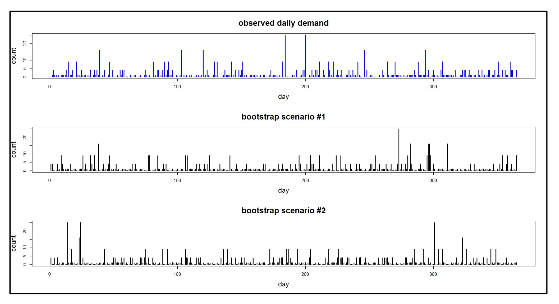
Figure 1: An observed demand sequence and demand scenarios derived from it.

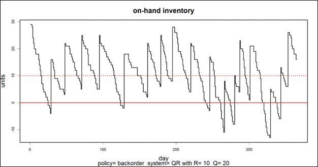
Figure 2 shows two demand scenarios and their consequences for stock on hand in a particular inventory control system. The difference between the two inventory plots illustrates the degree to which randomness in demand dominates the problem. The top plot shows two episodes of stockout, while the bottom plot shows nine. Averaging over many scenarios will clarify the typical values of Key Performance Metrics (KPIs) such as the average number of stockouts associated with any choice of Reorder Point and Order Quantity (which are 10 and 25, respectively, in Figure 2.)

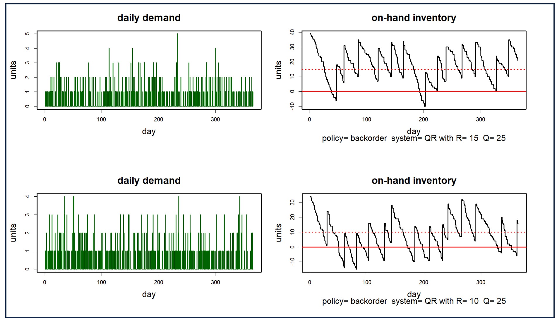
Figure 2: Two demand scenarios and their consequences for on-hand inventory

In this note, we’ll describe techniques for creating scenarios and list criteria for evaluating scenario generators.

Criteria for Scenarios

As we’ll see below, there are several ways to create scenarios. No matter the source, what criteria define a “good” scenario? There are four main criteria: fidelity, variety, quantity, and cost. Fidelity summarizes how accurately a scenario imitates real-world situations. High fidelity means the scenarios mirror actual events closely, providing a solid foundation for analysis and decision-making. Variety describes the diversity of scenarios a generator can create. A versatile generator can simulate a wide range of potential situations, allowing for a thorough exploration of possibilities and risks. Quantity refers to how many scenarios a generator can produce. A generator that can create a large number of scenarios provides ample data for analysis. Cost considers both the computational and human resources required to produce the scenarios. An efficient scenario generator balances quality with resource usage, ensuring the effort is justified by the value and accuracy of the outcomes.

Scenario Generation

Again, think of a scenario as a time series. How are scenarios created?

1. Geppetto’s Workshop: This approach involves hand-crafting scenarios manually by experts. While it can yield high fidelity (realism), it is very resource-intensive and cannot easily generate variety, which requires a large number of scenarios.
2. Groundhog Day: This method involves repeatedly using a single real-world situation as input. While it’s realistic by definition and cost-effective (no resources are used beyond recording the data), this approach lacks variety and so cannot accurately reflect the diversity of real-world scenarios.
3. Parametric Models: Examples of parametric models are the classics studied in Statistics 101 classes: the Normal, exponential, Poisson, etc. The demand plots in Figure 2 are generated parametrically, being the squares of Poisson random variables. These models generate an unlimited number of low cost scenarios having good variety, but they may not always capture the complexity of real-world data, potentially compromising fidelity. When reality is more complicated, these models generate over-simplified scenarios.
4. Non-Parametric Time Series Bootstraps: This approach can score well on all criteria: fidelity, variety, quantity, and cost. It’s a versatile method that excels in creating massive numbers of realistic scenarios. The synthetic demand histories in Figure 1 are simple bootstrap samples based on the observed values in the top graph. (For some nitty-gritty details about generating scenarios, see the links below.)

Exploiting Scenarios

Scenarios prove their worth in two ways: As inputs to decision making and as intuition-builders. For instance, when demand scenarios are used as inputs to simulation models, they enable stress testing and performance estimation for system design. Scenarios can also serve as intuition-builders for decision-makers or system operators. Their visual representation aids in developing insight into and appreciation for the risks involved in making operational decisions, be they for demand forecasting or inventory management.

Scenario-based analysis is very computer intensive, especially when the scenarios are generated by bootstrapping. At Smart Software, computation happens in the cloud. Imagine the computational load involved in determining reorder points and order quantities for each of tens of thousands of inventory items using hundreds or thousands of demand simulations for each item. Further imagine the software not only evaluating a specific proposed reorder point/order quantity pair but roaming over the entire “design space” of pairs to find the best pair of control parameters for each item. To make this practical, we take advantage of the parallel processing power of the cloud. Essentially, each inventory item is assigned its own computer to use in the calculations, so that all that computing can happen simultaneously rather than sequentially. Now we can cut loose and really get you the results you need.

Learning More

Those interested in further technical details and references can find more information here.

What Makes a Probabilistic Forecast?

Probabilistic Forecasting for Intermittent Demand

People new to the jobs of “demand planner” or “supply planner” are likely to have questions about the various forecasting terms and methods used in their jobs. This note may help by explaining these terms and showing how they relate.

Demand Planning

Demand planning is about how much of what you have to sell will go out the door in the future, e.g., how many what-nots you will sell next quarter. Here are six methodologies often used in demand planning.

• Statistical Forecasting
  • These methods use demand history to forecast future values. The two most common methods are curve fitting and data smoothing.
  • Curve fitting matches a simple mathematical function, like the equation for a straight line (y= a +b∙t) or an interest-rate type curve (y=a∙b^t), to the demand history. Then it extends that line or curve forward in time as the forecast.
  • In contrast, data smoothing does not result in an equation. Instead it sweeps through the demand history, averaging values along the way, to create a smoother version of the history. These methods are called exponential smoothing and moving average. In the simplest case (i.e., in the absence of trend or seasonality, for which variants exist), the goal is to estimate the current average level of demand and use that as the forecast.
  • These methods produce “point forecasts”, which are single-number estimates for each future time period (e.g., “Sales in March will be 218 units”). Sometimes they come with estimates of potential forecast error bolted on using separate models of demand variability (“Sales in March will be 218 ± 120 units”).

• Probabilistic Forecasting
  • This approach keys on the randomness of demand and works hard to estimate forecast uncertainty. It regards forecasting less as an exercise in cranking out specific numbers and more as an exercise in risk management.
  • It explicitly models the variability in demand and uses that to present results in the form of large numbers of scenarios constructed to show the full range of possible demand sequences. These are especially useful in tactical supply planning tasks, such as setting reorder points and order quantities.

• Causal Forecasting
  • Statistical forecasting models use as inputs only the past demand history of the item in question. They regard the up-and-down wiggles in the demand plot as the end result of myriad unnamed factors (interest rates, the price of tea in China, phases of the moon, whatever). Causal forecasting explicitly identifies one or more influences (interest rates, advertising spend, competitors’ prices, …) that could plausibly influence sales. Then it builds an equation relating the numerical values of these “drivers” or “causal factors” to item sales. The equation’s coefficients are estimated by “regression analysis”.

• Judgemental Forecasting
  • Golden Gut. Despite the general availability of gobs of data, some companies pay little attention to the numbers and give greater weight to the subjective judgements of an executive deemed to have a “Golden Gut”, which allows him or her to use “gut feel” to predict what future demand will be. If that person has great experience, has spent a career actually looking at the numbers, and is not prone to wishful thinking or other forms of cognitive bias, the Golden Gut can be a cheap, fast way to plan. But there is good evidence from studies of companies run this way that relying on the Golden Gut is risky.
  • Group Consensus. More common is a process that uses a periodic meeting to create a group consensus forecast. The group will have access to shared objective data and forecasts, but members will also have knowledge of factors that may not be measured well or at all, such as consumer sentiment or the stories relayed by sales reps. It is helpful to have a shared, objective starting point for these discussions consisting of some sort of objective statistical analysis. Then the group can consider adjusting the statistical forecast. This process anchors the forecast in objective reality but exploits all the other information available outside the forecasting database.
  • Scenario Generation. Sometimes several people will meet and discuss “strategic what-if” questions. “What if we lose our Australian customers?” “What if our new product roll-out is delayed by six months?” “What if our sales manager for the mid-west jumps to a competitor?” These bigger-picture questions can have implications for item-specific forecasts and might be added to any group-consensus forecasting meeting.

• New product forecasting
  • New products, by definition, have no sales history to support statistical, probability, or causal forecasting. Subjective forecasting methods can always be used here, but these often rely on a dangerous ratio of hopes to facts. Fortunately, there is at least partial support for objective forecasting in the form of curve fitting.
  • A graph of the cumulative sales of an item often describes some sort of “S-curve”, i.e., a graph that starts at zero, builds up, then levels off to a final lifetime total sales. The curve gets its name because it looks like a letter S somehow smeared and stretched to the right. Now there are an infinite number of S-curves, so forecasters typically pick an equation and subjectively specify some key parameter values, like when sales will hit 25%, 50% and 75% of total lifetime sales and what that final level will be. This is also overtly subjective, but it produces detailed period-by-period forecasts that can be updated as experience builds up. Finally, S-curves are sometimes shaped to match the known history of a similar, predecessor product (“Sales for our last gizmo looked like this, so let’s use that as a template.”).

Supply Planning

Demand planning feeds into supply planning by predicting future sales (e.g., for finished goods) or usage (e.g., for spare parts). Then it is up to supply planning to make sure the items in question will be available to sell or to use.

• Dependent demand
  • Dependent demand is demand that can be determined by its relationship to demand for another item. For instance, a bill of materials may show that a little red wagon consists of a body, a pull bar, four wheels, two axles, and various fasteners to keep the wheels on the axles and connect the pull bar to the body. So if you hope to sell 10 little red wagons, you’d better make 10, which means you need 10×2 = 20 axles, 10×4 = 40 wheels, etc. Dependent demand governs raw materials purchasing, component and subsystems purchasing, even personnel hiring (10 wagons need one high-school kid to put them together over a 1 hour shift).
  • If you have multiple products with partially overlapping bills of materials, you have a choice of two forecasting approaches. Suppose you sell not only little red wagons but little blue baby carriages and that both use the same axles. To predict the number of axles you need you could (1) predict the dependent demand for axles from each product and add the forecasts or (2) observe the total demand history for axles as its own time series and forecast that separately. Which works better is an empirical question that can be tested.

• Inventory management
  • Inventory management entails many different tasks. These include setting inventory control parameters such as reorder points and order quantities, reacting to contingencies such as stockouts and order expediting, setting staffing levels, and selecting suppliers.

• Forecasting plays a role in the first three. The number of replenishment orders that will be made in a year for each product determines how many people are needed to cut PO’s. The number and severity of stockouts in a year determines the number of contingencies that must be handled. The number of PO’s and stockouts in a year will be random but be governed by the choices of inventory control parameters. The implications of any such choices can be modeled by inventory simulations. These simulations will be driven by detailed demand scenarios generated by probabilistic forecasts.

​

Dealing with the day-to-day of inventory management can keep you busy. There’s the usual rhythm of ordering, receiving, forecasting and planning, and moving things around in the warehouse. Then there are the frenetic times – shortages, expedites, last-minute calls to find new suppliers.

All this activity works against taking a moment to see how you’re doing. But you know you have to get your head up now and then to see where you’re heading. For that, your inventory software should show you metrics – and not just one, but a full set of metrics or KPI’s – Key Performance Indicators.

Multiple Metrics

Depending on your role in your organization, different metrics will have different salience. If you are on the finance side of the house, inventory investment may be top of mind: how much cash is tied up in inventory? If you’re on the sales side, item availability may be top of mind: what’s the chance that I can say “yes” to an order? If you’re responsible for replenishment, how many PO’s will your people have to cut in the next quarter?

Availability Metrics

Let’s circle back to item availability. How do you put a number on that? The two most used availability metrics are “service level” and “fill rate.” What’s the difference? It’s the difference between saying “We had an earthquake yesterday” and saying, “We had an earthquake yesterday, and it was a 6.4 on the Richter scale.” Service level records the frequency of stockouts no matter their size; fill rate reflects their severity. The two can seem to point in opposite directions, which causes some confusion. You can have a good service level, say 90%, but have an embarrassing fill rate, say 50%. Or vice versa. What makes them different is the distribution of demand sizes. For instance, if the distribution is very skewed, so most demands are small but some are huge, you might get the 90%/50% split mentioned above. If your focus is on how often you have to backorder, service level is more relevant. If your worry is how big an overnight expedite can get, the fill rate is more relevant.

One Graph to Rule them All

A graph of on-hand inventory can provide the basis for calculating multiple KPI’s. Consider Figure 1, which plots on-hand each day for a year. This plot has information needed to calculate multiple metrics: inventory investment, service level, fill rate, reorder rate and other metrics.

Inventory investment: The average height of the graph when above zero, when multiplied by unit cost of the inventory item, gives quarterly dollar value.

Service level: The fraction of inventory cycles that end above zero is the service level. Inventory cycles are marked by the up movements occasioned by the arrival of replenishment orders.

Fill rate: The amount by which inventory drops below zero and how long it stays there combine to determine fill rate.

In this case, the average number of units on hand was 10.74, the service level was 54%, and the fill rate was 91%.

KPI’s and KPP’s

In the over forty years since we founded Smart Software, I have never seen a customer produce a plot like Figure 1.  Those who are further along in their development do produce and pay attention to reports listing their KPI’s in tabular form, but they don’t look at such a graph. Nevertheless, that graph has value for developing insight into the random rhythms of inventory as it rises and falls.

Where it is especially useful is prospectively. Given market volatility, key variables like supplier lead times, average demand, and demand variability all shift over time. This implies that key control parameters like reorder points and order quantities must adjust to these shifts. For instance, if a supplier says they’ll have to increase their average lead time by 2 days, this will impact your metrics negatively, and you may need to increase your reorder point to compensate. But increase it by how much?

Here is where modern inventory software comes in. It will let you propose an adjustment and then see how things will play out. Plots like Figure 1 let you see and get a feel for the new regime. And the plots can be analyzed to compute KPP’s – Key Performance Predictions.

KPP’s help take the guesswork out of adjustments. You can simulate what will happen to your KPI’s if you change them in response to changes in your operating environment – and how bad things will get if you make no changes.

Are you confused about what is AI and what is machine learning? Are you unsure why knowing more will help you with your job in inventory planning? Don’t despair. You’ll be ok, and we’ll show you how some of whatever-it-is can be useful.

What is and what isn’t

What is AI and how does it differ from ML? Well, what does anybody do these days when they want to know something? They Google it. And when they do, the confusion starts.

One source says that the neural net methodology called deep learning is a subset of machine learning, which is a subset of AI. But another source says that deep learning is already a part of AI because it sort of mimics the way the human mind works, while machine learning doesn’t try to do that.

One source says there are two types of machine learning: supervised and unsupervised. Another says there are four: supervised, unsupervised, semi-supervised and reinforcement.

Some say reinforcement learning is machine learning; others call it AI.

Some of us traditionalists call a lot of it “statistics”, though not all of it is.

In the naming of methods, there is a lot of room for both emotion and salesmanship. If a software vendor thinks you want to hear the phrase “AI”, they may well say it for you just to make you happy.

Better to focus on what comes out at the end

You can avoid some confusing hype if you focus on the end result you get from some analytic technology, regardless of its label. There are several analytical tasks that are relevant to inventory planners and demand planners. These include clustering, anomaly detection, regime change detection, and regression analysis. All four methods are usually, but not always, classified as machine learning methods. But their algorithms can come straight out of classical statistics.

Clustering

Clustering means grouping together things that are similar and distancing them from things that are dissimilar. Sometimes clustering is easy: to separate your customers geographically, simply sort them by state or sales region. When the problem is not so dead obvious, you can use data and clustering algorithms to get the job done automatically even when dealing with massive datasets.

For example, Figure 1 illustrates a cluster of “demand profiles”, which in this case divides all a customer’s items into nine clusters based on the shape of their cumulative demand curves. Cluster 1.1 in the top left contains items whose demand has been petering out, while Cluster 3.1 in the bottom left contains items whose demand has accelerated.  Clustering can also be done on suppliers. The choice of number of clusters is typically left to user judgement, but ML can guide that choice.  For example, a user might instruct the software to “break my parts into 4 clusters” but using ML may reveal that there are really 6 distinct clusters the user should analyze. 

Figure 1: Clustering items based on the shapes of their cumulative demand

Anomaly Detection

Demand forecasting is traditionally done using time series extrapolation. For instance, simple exponential smoothing works to find the “middle” of the demand distribution at any time and project that level forward. However, if there has been a sudden, one-time jump up or down in demand in the recent past, that anomalous value can have a significant but unwelcome effect on the near-term forecast.  Just as serious for inventory planning, the anomaly can have an outsized effect on the estimate of demand variability, which goes directly to the calculation of safety stock requirements.

Planners may prefer to find and remove such anomalies (and maybe do offline follow-up to find out the reason for the weirdness). But nobody with a big job to do will want to visually scan thousands of demand plots to spot outliers, expunge them from the demand history, then recalculate everything. Human intelligence could do that, but human patience would soon fail. Anomaly detection algorithms could do the work automatically using relatively straightforward statistical methods. You could call this “artificial intelligence” if you wish.

Regime Change Detection

Regime change detection is like the big brother of anomaly detection. Regime change is a sustained, rather than temporary, shift in one or more aspects of the character of a time series. While anomaly detection usually focuses on sudden shifts in mean demand, regime change could involve shifts in other features of the demand, such as its volatility or its distributional shape.  

Figure 2 illustrates an extreme example of regime change. The bottom dropped out of demand for this item around day 120. Inventory control policies and demand forecasts based on the older data would be wildly off base at the end of the demand history.

Figure 2: An example of extreme regime change in an item with intermittent demand

Here too, statistical algorithms can be developed to solve this problem, and it would be fair play to call them “machine learning” or “artificial intelligence” if so motivated.  Using ML or AI to identify regime changes in demand history enables demand planning software to automatically use only the relevant history when forecasting instead of having to manually pick the amount of history to introduce to the model. 

Regression analysis

Regression analysis relates one variable to another through an equation. For example, sales of window frames in one month may be predicted from building permits issued a few months earlier. Regression analysis has been considered a part of statistics for over a century, but we can say it is “machine learning” since an algorithm works out the precise way to convert knowledge of one variable into a prediction of the value of another.

Summary

It is reasonable to be interested in what’s going on in the areas of machine learning and artificial intelligence. While the attention given to ChatGPT and its competitors is interesting, it is not relevant to the numerical side of demand planning or inventory management. The numerical aspects of ML and AI are potentially relevant, but you should try to see through the cloud of hype surrounding these methods and focus on what they can do.  If you can get the job done with classical statistical methods, you might just do that, then exercise your option to stick the ML label on anything that moves.

Forecasting inventory requirements is a specialized variant of forecasting that focuses on the high end of the range of possible future demand.

For simplicity, consider the problem of forecasting inventory requirements for just one period ahead, say one day ahead. Usually, the forecasting job is to estimate the most likely or average level of product demand. However, if available inventory equals the average demand, there is about a 50% chance that demand will exceed inventory and result in lost sales and/or lost good will. Setting the inventory level at, say, ten times the average demand will probably eliminate the problem of stockouts, but will just as surely result in bloated inventory costs.

The trick of inventory optimization is to find a satisfactory balance between having enough inventory to meet most demand without tying up too many resources in the process. Usually, the solution is a blend of business judgment and statistics. The judgmental part is to define an acceptable inventory service level, such as meeting 95% of demand immediately from stock. The statistical part is to estimate the 95th percentile of demand.

When not dealing with intermittent demand, you can often estimate the required inventory level by assuming a bell-shaped (Normal) curve of demand, estimating both the middle and the width of the bell curve, then using a standard statistical formula to estimate the desired percentile. The difference between the desired inventory level and the average level of demand is called the “safety stock” because it protects against the possibility of stockouts.

When dealing with intermittent demand, the bell-shaped curve is a very poor approximation to the statistical distribution of demand. In this special case, Smart leverages patented technology for intermittent demand that is designed to accurately forecast the ranges and produce a better estimate of the safety stock needed to achieve the required inventory service level.