A forecast is a prediction about the value of a time series variable at some time in the future. For instance, one might want to estimate next month’s sales or demand for a product item. A time series is a sequence of numbers recorded at equally spaced time intervals; for example, unit sales recorded every month.

The objectives you pursue when you forecast depend on the nature of your job and your business. Every forecast is uncertain; in fact, there is a range of possible values for any variable you forecast. Values near the middle of this range have a higher likelihood of actually occurring, while values at the extremes of the range are less likely to occur. The following figure illustrates a typical distribution of forecast values.

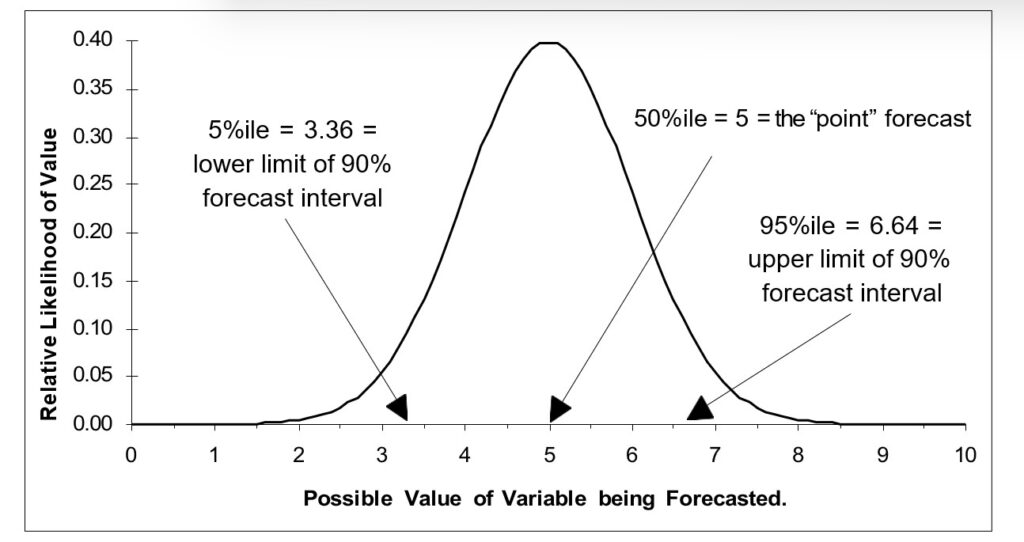
Illustrating a forecast distribution of forecast values

Point forecasts

The most common use of forecasts is to estimate a sequence of numbers representing the most likely future values of the variable of interest. For instance, suppose you are developing a sales and marketing plan for your company. You may need to fill in 12 cells in a financial spreadsheet with estimates of your company’s total revenues over the next 12 months. Such estimates are called point forecasts because you want a single number (data point) for each forecast period. Smart Demand Planner’ Automatic forecasting feature provides you with these point forecasts automatically.

Interval forecasts

Although point forecasts are convenient, you will often benefit more from interval forecasts. Interval forecasts show the most likely range (interval) of values that might arise in the future. These are usually more useful than point forecasts because they convey the amount of uncertainty or risk involved in a forecast. The forecast interval percentage can be specified in the various forecasting dialog boxes in the Demand Planning Software.  Each of the many forecasting methods (automatic, moving average, exponential smoothing and so on) available in Smart Demand Planner allow you to set a forecast interval.

The default configuration in Smart Demand Planner provides 90% forecast intervals. Interpret these intervals as the range within which the actual values will fall 90% of the time. If the intervals are wide, then there is a great deal of uncertainty associated with the point forecasts. If the intervals are narrow, you can be more confident. If you are performing a planning function and want best case and worst case values for the variables of interest at several times in the future, you can use the upper and lower limits of the forecast intervals for that purpose, with the single point estimate providing the most likely value. In the previous figure, the 90% forecast interval extends from 3.36 to 6.64.

Upper percentiles

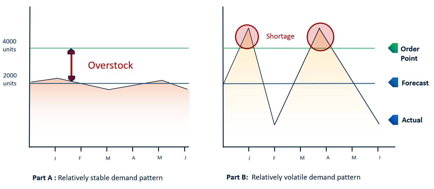
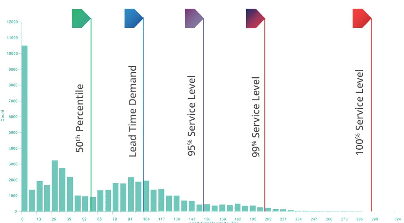
In inventory control, your goal may be to make good estimates of a high percentile of the demand for a product item. These estimates help you cope with the tradeoff between, on the one hand, minimizing the costs of holding and ordering stock, and, on the other hand, minimizing the number of lost or back-ordered sales due to a stock out. For this reason, you may wish to know the 99th percentile or service level of demand, since the chance of exceeding that level is only 1%.

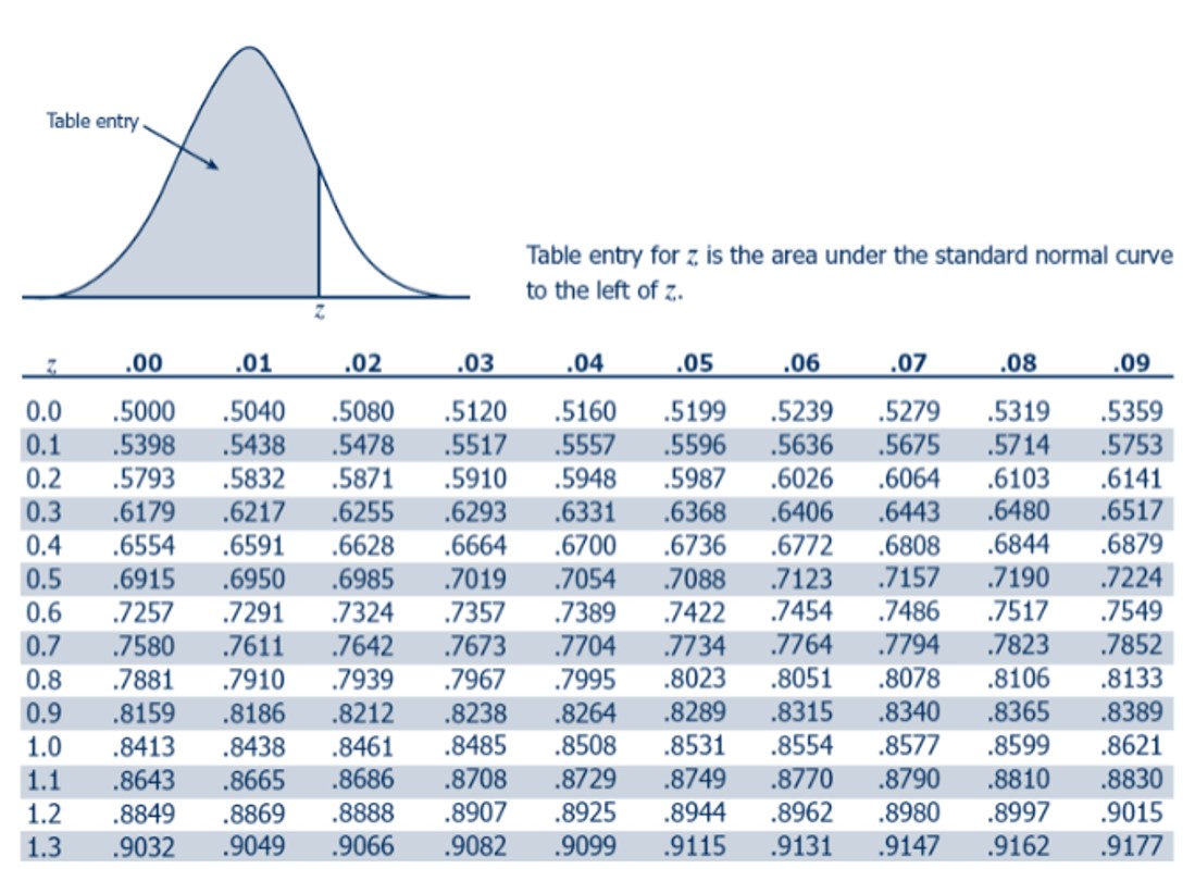
When forecasting individual variables with features like Automatic forecasting, note that the upper limit of a 90% forecast interval represents the 95th percentile of the predicted distribution of the demand for that variable. (Subtracting the 5th percentile from the 95th percentile leaves an interval containing 95%-5% = 90% of the possible values.) This means you can estimate upper percentiles by changing the value of the forecast interval. In the figure, “Illustrating a forecast distribution”, the 95th percentile is 6.64.

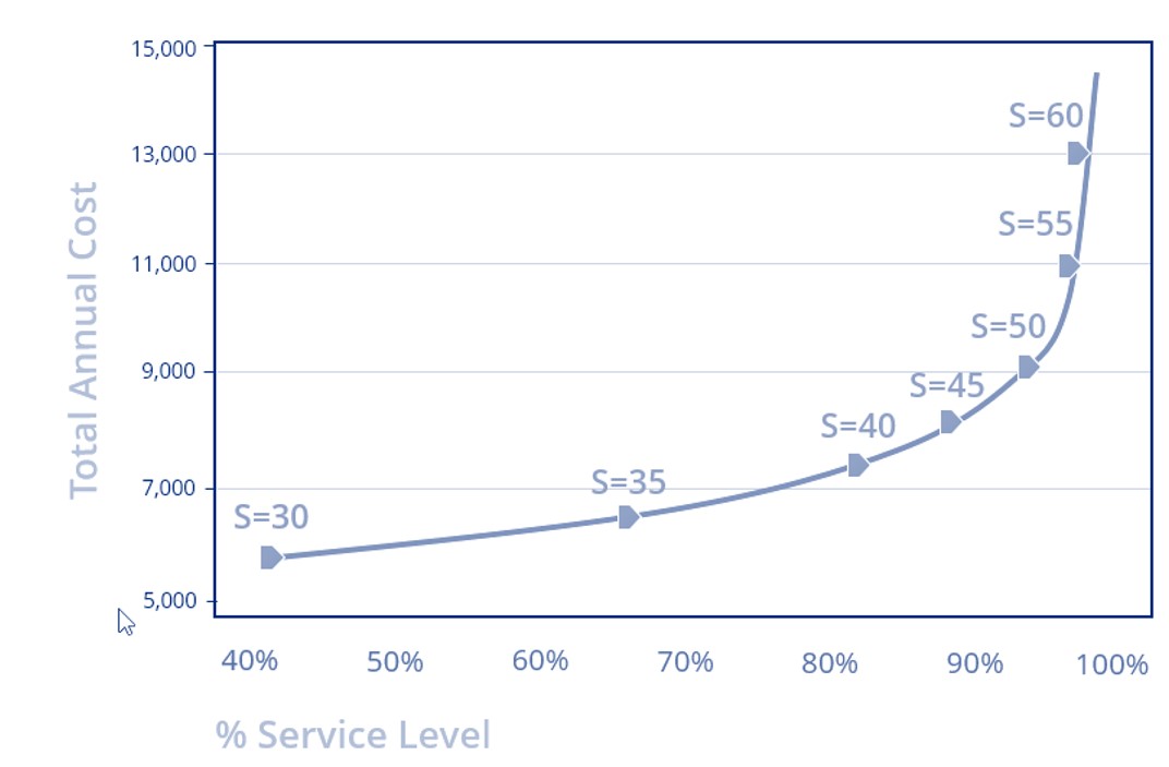
To optimize stocking policies at the desired service level or to let the system recommend which stocking policy and service level generates the best return, consider using Smart Inventory Optimization.   It is designed to support what-if scenarios that show predicted tradeoffs of varying inventory polices including different service level targets.

Lower percentiles

Sometimes you may be concerned with the lower end of the predicted distribution for a variable. Such cases often arise in financial applications, where a low percentile of a revenue estimate represents a contingency requiring financial reserves. You can use Smart Demand Planner in this case in a way analogous to the case of forecasting upper percentiles. In the figure, “Illustrating a forecast distribution” , the 5th percentile is 3.36.

In conclusion, forecasting involves predicting future values, with point forecasts offering single estimates and interval forecasts providing likely value ranges. Smart Demand Planner automates point forecasts and allows users to set intervals, aiding in uncertainty assessment. For inventory control, the tool facilitates understanding upper (e.g., 99th percentile) and lower (e.g., 5th percentile) percentiles. To optimize stocking policies and service levels, Smart Inventory Optimization supports what-if scenarios, ensuring effective decision-making on how much to stock given the risk of stock out you are willing to accept.

Lead time delays and supply variability are supply chain facts of life, yet inventory-carrying organizations are often caught by surprise when a supplier is late. An effective inventory planning process embraces this fact of life and develops policies that effectively account for this uncertainty. Sure, there will be times when lead time delays come out of nowhere and cause a shortage. But most often, the shortages result from:

1. Not computing stocking policies (e.g., reorder points, safety stocks, and Min/Max levels) often enough to catch changes in the lead time. 
2. Using poor estimates of actual lead time such as using only averages of historical receipts or relying on a supplier quote.

Instead, recalibrate policies across every single part during every planning cycle to catch changes in demand and lead times.  Rather than assuming only an average lead time, simulate the lead times using scenarios.  This way, recommended stocking policies account for the probabilities of lead times being high and adjust accordingly.  When you do this, you’ll identify needed inventory increases before it is too late. You’ll capture more sales and drive significant improvements in customer satisfaction.

Summary

Smart Software’s advanced supply chain analytics exploits multiple advanced methods. Two of the most important are “statistical bootstrapping” and “Monte Carlo simulation”. Since both involve lots of random numbers flying around, folks sometimes get confused about which is which and what they are good for. Hence, this note. Bottom line up front: Statistical bootstrapping generates demand scenarios for forecasting. Monte Carlo simulation uses the scenarios for inventory optimization.

Bootstrapping

Bootstrapping, also called “resampling” is a method of computational statistics that we use to create demand scenarios for forecasting. The essence of the forecasting problem is to expose possible futures that your company might confront so you can work out how to manage business risks. Traditional forecasting methods focus on computing “most likely” futures, but they fall short of presenting the full risk picture. Bootstrapping provides an unlimited number of realistic what-if scenarios.

Bootstrapping does this without making unrealistic assumptions about the demand, i.e., that it is not intermittent, or that it has a bell-shaped distribution of sizes. Those assumptions are crutches to make the math simpler, but the bootstrap is a procedure,  not an equation, so it doesn’t need such simplifications.

For the simplest demand type, which is a stable randomness with no seasonality or trend, bootstrapping is dead easy. To get a reasonable idea of what a single future demand value might be, pick one of the historical demands at random. To create a demand scenario, make multiple random selections from the past and string them together. Done. It is possible to add a little more realism by “jittering” the demand values, i.e., adding or subtracting a bit of additional randomness to each one, but even that is simple.

Figure 1 shows a simple bootstrap. The first line is a short sequence of historical demand for an SKU. The following lines show scenarios of future demand created by randomly selecting values from the demand history. For instance, the next three demand might be (0, 14, 6), or (2, 3, 5), etc.

Figure 1: Example of demand scenarios generated by a simple bootstrap

Higher frequency operations such as daily forecasting bring with them more complex demand patterns, such as double seasonality (e.g., day-of-week and month-of-year) and/or trend. This challenged us to invent a new generation of bootstrapping algorithms. We recently won a US Patent for this breakthrough, but the essence is as described above.

Monte Carlo Simulation

Monte Carlo is famous for its casinos, which, like bootstrapping, invoke the idea of randomness. Monte Carlo methods go back a long way, but the modern impetus came with the need to do some hairy calculations about where neutrons would fly when an A-bomb explodes.

The essence of Monte Carlo analysis is this: “Our problem is too complicated to analyze with paper-and-pencil equations. So, let’s write a computer program that codes the individual steps of the process, put in the random elements (e.g., which way a neutron shoots away), wind it up and watch it go. Since there’s a lot of randomness, let’s run the program a zillion times and average the results.”

Applying this approach to inventory management, we have a different set of randomly occurring events: e.g., a demand of a given size arrives on a random day, a replenishment of a given size arrives after a random lead time, we cut a replenishment PO of a given size when stock drops to or below a given reorder point. We code the logic relating these events into a program. We feed it with a random demand sequence (see bootstrapping above), run the program for a while, say one year of daily operations, compute performance metrics like Fill Rate and Average On Hand inventory, and “toss the dice” by re-running the program many times and averaging the results of many simulated years. The result is a good estimate of what happens when we make key management decisions: “If we set the reorder point at 10 units and the order quantity at 15 units, we can expect to get a service level of 89% and an average on hand of 21 units.” What the simulation is doing for us is exposing the consequences of management decisions based on realistic demand scenarios and solid math. The guesswork is gone.

Figure 2 shows some of the inner workings of a Monte Carlo simulation of an inventory system in four panels. The system uses a Min/Max inventory control policy with Min=10 and Max=25. No backorders are allowed: you have the good or you lose the business. Replenishment lead times are usually 7 days but sometimes 14. This simulation ran for one year.

The first panel shows a complex random demand scenario in which there is no demand on weekends, but demand generally increases each day from Monday to Friday. The second panel shows the random number of units on hand, which ebbs and flows with each replenishment cycle. The third panel shows the random sizes and timings of replenishment orders coming in from the supplier. The final panel shows the unsatisfied demand that jeopardizes customer relationships. This kind of detail can be very useful for building insight into the dynamics of an inventory system.

Figure 2: Details of a Monte Carlo simulation

Figure 2 shows only one of the countless ways that the year could play out. Generally, we want to average the results of many simulated years. After all, nobody would flip a coin once to decide if it were a fair coin. Figure 3 shows how four key performance metrics (KPI’s) vary from year to year for this system. Some metrics are relatively stable across simulations (Fill Rate), but others show more relative variability (Operating Cost= Holding Cost + Ordering Cost + Shortage Cost). Eyeballing the plots, we can estimate that the choices of Min=10, Max=25 leads to an average Operating cost of around $3,000 per year, a Fill Rate of around 90%, a Service Level of around 75%, and an Average On Hand of about 10

Figure 3: Variation in KPI’s computed over 1,000 simulated years

In fact, it is now possible to answer a higher level of management question. We can go beyond “What will happen if I do such-and-such?” to “What is the best thing I can do to achieve a fill rate of at least 90% for this item at the lowest possible cost?” The mathemagic  behind this leap is yet another key technology called “stochastic optimization”, but we’ll stop here for now. Suffice it to say that Smart’s SIO&P software can search the “design space” of Min and Max values to automatically find the best choice.

Managing spare parts presents numerous challenges, such as unexpected breakdowns, changing schedules, and inconsistent demand patterns. Traditional forecasting methods and manual approaches are ineffective in dealing with these complexities. To overcome these challenges, this blog outlines key strategies that prioritize service levels, utilize probabilistic methods to calculate reorder points, regularly adjust stocking policies, and implement a dedicated planning process to avoid excessive inventory. Explore these strategies to optimize spare parts inventory and improve operational efficiency.

Bottom Line Upfront

​1.Inventory Management is Risk Management.

2.Can’t manage risk well or at scale with subjective planning – Need to know service vs. cost.

3.It’s not supply & demand variability that are the problem – it’s how you handle it.

4.Spare parts have intermittent demand so traditional methods don’t work.

5.Rule of thumb approaches don’t account for demand variability and misallocate stock.

6.Use Service Level Driven Planning  (service vs. cost tradeoffs) to drive stock decisions.

7.Probabilistic approaches such as bootstrapping yield accurate estimates of reorder points.

8.Classify parts and assign service level targets by class.

9.Recalibrate often – thousands of parts have old, stale reorder points.

10.Repairable parts require special treatment.

Do Focus on the Real Root Causes

Intermittent Demand

• Slow moving, irregular or sporadic with a large percentage of zero values.
• Non-zero values are mixed in randomly – spikes are large and varied.
• Isn’t bell shaped (demand is not Normally distributed around the average.)
• At least 70% of a typical Utility’s parts are intermittently demanded.

Normal Demand

• Very few periods of zero demand (exception is seasonal parts.)
• Often exhibits trend, seasonal, or cyclical patterns.
• Lower levels of demand variability.
• Is bell-shaped (demand is Normally distributed around the average.)

Don’t rely on averages

• OK for determining typical usage over longer periods of time.
• Often forecasts more “accurately” than some advanced methods.
• But…insufficient for determining what to stock.

Don’t Buffer with Multiples of Averages

Example:  Two equally important parts so let’s treat them the same.
We’ll order more  when On Hand Inventory ≤ 2 x Avg Lead Time Demand.

Do use Service Level tradeoff curves to compute safety stock

Standard Normal Probabilities

OK for normal demand. Doesn’t work with intermittent demand!

Don’t use Normal (Bell Shaped) Distributions

• You’ll get the tradeoff curve wrong:

– e.g., You’ll target 95% but achieve 85%.

– e.g., You’ll target 99% but achieve 91%.

• This is a huge miss with costly implications:

– You’ll stock out more often than expected.

– You’ll start to add subjective buffers to compensate and then overstock.

– Lack of trust/second-guessing of outputs paralyzes planning.

Why Traditional Methods Fail on Intermittent Demand: 

Traditional Methods are not designed to address core issues in spare parts management.

Need: Probability distribution (not bell-shaped) of demand over variable lead time.

• Get: Prediction of average demand in each month, not a total over lead time.
• Get: Bolted-on model of variability, usually the Normal model, usually wrong.

Need: Exposure of tradeoffs between item availability and cost of inventory.

• Get: None of this; instead, get a lot of inconsistent, ad-hoc decisions.

Do use Statistical Bootstrapping to Predict the Distribution:

Then exploit the distribution to optimize stocking policies.

How does Bootstrapping Work?

24 Months of Historical Demand Data.

Bootstrap Scenarios for a 3-month Lead Time.

Bootstrapping Hits the Service Level Target with nearly 100% Accuracy!

• National Warehousing Operation.

Task: Forecast inventory stocking levels for 12,000 intermittently demanded SKUs at 95% & 99% service levels

Results:

At 95% service level, 95.23% did not stock out.

At 99% service level, 98.66% did not stock out.

This means you can rely on output to set expectations and confidently make targeted stock adjustments that lower inventory and increase service.

Set Target Service Levels According to Order Frequency & Size

Recalibrate Reorder Points Frequently

• Static ROPs cause excess and shortages.
• As lead time increases, so should the ROP and vice versa.
• As usage decreases, so should the ROP and vice versa.
• Longer you wait to recalibrate, the greater the imbalance.
• Mountains of parts ordered too soon or too late.
• Wastes buyers’ time placing the wrong orders.
• Breeds distrust in systems and forces data silos.

Do Plan Rotables (Repair Parts) Differently

Summary

1.Inventory Management is Risk Management.

2.Can’t manage risk well or at scale with subjective planning – Need to know service vs. cost.

3.It’s not supply & demand variability that are the problem – it’s how you handle it.

4.Spare parts have intermittent demand so traditional methods don’t work.

5.Rule of thumb approaches don’t account demand variability and misallocate stock.

6.Use Service Level Driven Planning  (service vs. cost tradeoffs) to drive stock decisions.

7.Probabilistic approaches such as bootstrapping yield accurate estimates of reorder points.

8.Classify parts and assign service level targets by class.

9.Recalibrate often – thousands of parts have old, stale reorder points.

10.Repairable parts require special treatment.

Belmont, MA, June 2023 – Smart Software, Inc., provider of industry-leading demand forecasting, planning, and inventory optimization solutions, today announced the award of US Patent 11,656,887, “SYSTEM AND METHOD TO SIMULATE DEMAND AND OPTIMIZE CONTROL PARAMETERS FOR A TECHNOLOGY PLATFORM.”

The patent directs “technical solutions for analyzing historical demand data of resources in a technology platform to facilitate management of an automated process in the platform.” One important application is optimization of parts inventories.

Aspects of the invention include: an advanced bootstrap process that converts a single observed time series of item demand into an unlimited number of realistic demand scenarios; a performance prediction process that executes Monte Carlo simulations of a proposed inventory control policy to assess its performance; and a performance improvement process that uses the performance prediction process to automatically explore the space of alternative system designs to identify optimal control parameter values, selecting ones that minimize operating cost while guaranteeing a target level of item availability.

The new analytic technology described in the patent will form the basis for the upcoming release of the next generation (“Gen2”) of Smart Demand Planner™ and Smart IP&O™. Current customers and resellers can preview Gen2 by contacting their Smart Software sales representative.

Research underlying the patent was self-funded by Smart, supplemented by competitive Small Business Innovation Research grants from the US National Science Foundation.

About Smart Software, Inc.
Founded in 1981, Smart Software, Inc. is a leader in providing businesses with enterprise-wide demand forecasting, planning, and inventory optimization solutions.  Smart Software’s demand forecasting and inventory optimization solutions have helped thousands of users worldwide, including customers such as Disney, Arizona Public Service, Ameren, and The American Red Cross.  Smart’s Inventory Planning & Optimization Platform, Smart IP&O gives demand planners the tools to handle sales seasonality, promotions, new and aging products, multi-dimensional hierarchies, and intermittently demanded service parts and capital goods items.  It also provides inventory managers with accurate estimates of the optimal inventory and safety stock required to meet future orders and achieve desired service levels.  Smart Software is headquartered in Belmont, Massachusetts, and our website is www.smartcorp.com.