Can Randomness be an Ally in the Forecasting Battle?

Feynman’s perspective illuminates our journey:  “In its efforts to learn as much as possible about nature, modern physics has found that certain things can never be “known” with certainty. Much of our knowledge must always remain uncertain. The most we can know is in terms of probabilities.” ― Richard Feynman, The Feynman Lectures on Physics.

When we try to understand the complex world of logistics, randomness plays a pivotal role. This introduces an interesting paradox: In a reality where precision and certainty are prized, could the unpredictable nature of supply and demand actually serve as a strategic ally?

The quest for accurate forecasts is not just an academic exercise; it’s a critical component of operational success across numerous industries. For demand planners who must anticipate product demand, the ramifications of getting it right—or wrong—are critical. Hence, recognizing and harnessing the power of randomness isn’t merely a theoretical exercise; it’s a necessity for resilience and adaptability in an ever-changing environment.

Embracing Uncertainty: Dynamic, Stochastic, and Monte Carlo Methods

Dynamic Modeling: The quest for absolute precision in forecasts ignores the intrinsic unpredictability of the world. Traditional forecasting methods, with their rigid frameworks, fall short in accommodating the dynamism of real-world phenomena. By embracing uncertainty, we can pivot towards more agile and dynamic models that incorporate randomness as a fundamental component. Unlike their rigid predecessors, these models are designed to evolve in response to new data, ensuring resilience and adaptability. This paradigm shift from a deterministic to a probabilistic approach enables organizations to navigate uncertainty with greater confidence, making informed decisions even in volatile environments.

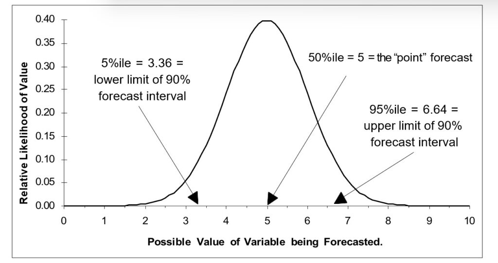
Stochastic modeling guides forecasters through the fog of unpredictability with the principles of probability. Far from attempting to eliminate randomness, stochastic models embrace it. These models eschew the notion of a singular, predetermined future, presenting instead an array of possible outcomes, each with its estimated probability. This approach offers a more nuanced and realistic representation of the future, acknowledging the inherent variability of systems and processes. By mapping out a spectrum of potential futures, stochastic modeling equips decision-makers with a comprehensive understanding of uncertainty, enabling strategic planning that is both informed and flexible.

Named after the historical hub of chance and fortune, Monte Carlo simulations harness the power of randomness to explore the vast landscape of possible outcomes. This technique involves the generation of thousands, if not millions, of scenarios through random sampling, each scenario painting a different picture of the future based on the inherent uncertainties of the real world. Decision-makers, armed with insights from Monte Carlo simulations, can gauge the range of possible impacts of their decisions, making it an invaluable tool for risk assessment and strategic planning in uncertain environments.

Real-World Successes: Harnessing Randomness

The strategy of integrating randomness into forecasting has proven invaluable across diverse sectors. For instance, major investment firms and banks constantly rely on stochastic models to cope with the volatile behavior of the stock market. A notable example is how hedge funds employ these models to predict price movements and manage risk, leading to more strategic investment choices.

Similarly, in supply chain management, many companies rely on Monte Carlo simulations to tackle the unpredictability of demand, especially during peak seasons like the holidays. By simulating various scenarios, they can prepare for a range of outcomes, ensuring that they have adequate stock levels without overcommitting resources. This approach minimizes the risk of both stockouts and excess inventory.

These real-world successes highlight the value of integrating randomness into forecasting endeavors. Far from being the adversary it’s often perceived to be, randomness emerges as an indispensable ally in the intricate ballet of forecasting. By adopting methods that honor the inherent uncertainty of the future—bolstered by advanced tools like Smart IP&O—organizations can navigate the unpredictable with confidence and agility. Thus, in the grand scheme of forecasting, it may be wise to embrace the notion that while we cannot control the roll of the dice, we can certainly strategize around it.


The Objectives in Forecasting

A forecast is a prediction about the value of a time series variable at some time in the future. For instance, one might want to estimate next month’s sales or demand for a product item. A time series is a sequence of numbers recorded at equally spaced time intervals; for example, unit sales recorded every month.

The objectives you pursue when you forecast depend on the nature of your job and your business. Every forecast is uncertain; in fact, there is a range of possible values for any variable you forecast. Values near the middle of this range have a higher likelihood of actually occurring, while values at the extremes of the range are less likely to occur. The following figure illustrates a typical distribution of forecast values.

forecast distribution of forecast values

Illustrating a forecast distribution of forecast values


Point forecasts

The most common use of forecasts is to estimate a sequence of numbers representing the most likely future values of the variable of interest. For instance, suppose you are developing a sales and marketing plan for your company. You may need to fill in 12 cells in a financial spreadsheet with estimates of your company’s total revenues over the next 12 months. Such estimates are called point forecasts because you want a single number (data point) for each forecast period. Smart Demand Planner’ Automatic forecasting feature provides you with these point forecasts automatically.

Interval forecasts

Although point forecasts are convenient, you will often benefit more from interval forecasts. Interval forecasts show the most likely range (interval) of values that might arise in the future. These are usually more useful than point forecasts because they convey the amount of uncertainty or risk involved in a forecast. The forecast interval percentage can be specified in the various forecasting dialog boxes in the Demand Planning SoftwareEach of the many forecasting methods (automatic, moving average, exponential smoothing and so on) available in Smart Demand Planner allow you to set a forecast interval.

The default configuration in Smart Demand Planner provides 90% forecast intervals. Interpret these intervals as the range within which the actual values will fall 90% of the time. If the intervals are wide, then there is a great deal of uncertainty associated with the point forecasts. If the intervals are narrow, you can be more confident. If you are performing a planning function and want best case and worst case values for the variables of interest at several times in the future, you can use the upper and lower limits of the forecast intervals for that purpose, with the single point estimate providing the most likely value. In the previous figure, the 90% forecast interval extends from 3.36 to 6.64.

Upper percentiles

In inventory control, your goal may be to make good estimates of a high percentile of the demand for a product item. These estimates help you cope with the tradeoff between, on the one hand, minimizing the costs of holding and ordering stock, and, on the other hand, minimizing the number of lost or back-ordered sales due to a stock out. For this reason, you may wish to know the 99th percentile or service level of demand, since the chance of exceeding that level is only 1%.

When forecasting individual variables with features like Automatic forecasting, note that the upper limit of a 90% forecast interval represents the 95th percentile of the predicted distribution of the demand for that variable. (Subtracting the 5th percentile from the 95th percentile leaves an interval containing 95%-5% = 90% of the possible values.) This means you can estimate upper percentiles by changing the value of the forecast interval. In the figure, “Illustrating a forecast distribution”, the 95th percentile is 6.64.

To optimize stocking policies at the desired service level or to let the system recommend which stocking policy and service level generates the best return, consider using Smart Inventory Optimization.   It is designed to support what-if scenarios that show predicted tradeoffs of varying inventory polices including different service level targets.

Lower percentiles

Sometimes you may be concerned with the lower end of the predicted distribution for a variable. Such cases often arise in financial applications, where a low percentile of a revenue estimate represents a contingency requiring financial reserves. You can use Smart Demand Planner in this case in a way analogous to the case of forecasting upper percentiles. In the figure, “Illustrating a forecast distribution” , the 5th percentile is 3.36.

In conclusion, forecasting involves predicting future values, with point forecasts offering single estimates and interval forecasts providing likely value ranges. Smart Demand Planner automates point forecasts and allows users to set intervals, aiding in uncertainty assessment. For inventory control, the tool facilitates understanding upper (e.g., 99th percentile) and lower (e.g., 5th percentile) percentiles. To optimize stocking policies and service levels, Smart Inventory Optimization supports what-if scenarios, ensuring effective decision-making on how much to stock given the risk of stock out you are willing to accept.