We often encounter Excel-based reorder point planning methods.  In this post, we’ve detailed an approach that a customer used prior to proceeding with Smart.  We describe how their spreadsheet worked, the statistical approaches it relied on, the steps planners went through each planning cycle, and their stated motivations for using (and really liking) this internally developed spreadsheet.

Their monthly process consisted of updating a new month of actuals into the “reorder point sheet.”  An embedded formula recomputed the Reorder Point (ROP) and order-up-to (Max) level.  It worked like this:

• ROP = LT Demand + Safety Stock
• LT Demand = average daily demand x lead time days (assumed constant to keep things simple)
• Safety Stock for long lead time parts = Standard deviation x 2.0
• Safety Stock for short lead time parts = Standard deviation x 1.2
• Max = ROP + supplier-dictated Minimum Order Quantity

Historical averages and standard deviations used 52-weeks of rolling history (i.e., the newest week replaced the oldest week each period).  The standard deviation of demand was computed using the “stdevp” function in Excel.

Every month, a new ROP was recomputed. Both the average demand and standard deviation were modified by the new week’s demand, which in turn updated the ROP.

The default ROP is always based on the above logic. However, planners would make changes under certain conditions:

1. Planners would increase the Min for inexpensive parts to reduce risk of taking an on-time delivery hit (OTD) on an inexpensive part.

2. The Excel sheet identified any part with a newly calculated ROP that was ± 20% different from the current ROP.

3. Planners reviewed parts that exceed the exception threshold, proposed changes, and got a manager to approve.

4. Planners reviewed items with OTD hits and increased the ROP based on their intuition. Planners continued to monitor those parts for several periods and lowered the ROP when they felt it is safe.

5. Once the ROP and Max quantity were determined, the file of revised results was sent to IT, who uploaded into their ERP.

6. The ERP system then managed daily replenishment and order management.

Objectively, this was perhaps an above-average approach to inventory management. For instance, some companies are unaware of the link between demand variability and safety stock requirements and rely on rule of methods or intuition exclusively.  However,  there are problems with their approach:

1. Manual data updates
The spreadsheets required manual updating. To recompute, multiple steps were required, each with their own dependency. First, a data dump needed to be run from the ERP system.  Second, a planner would need to open the spreadsheet and review it to make sure the data imported properly.  Third, they needed to review output to make sure it calculated as expected.  Fourth, manual steps were required to push the results back to the ERP system.

2. One Size Fits All Safety Stock
Or in this case, “one of two sizes fit all”. The choice of using 2x and 1.2x standard deviation for long and short lead time items respectively equates to service levels of 97.7% and 88.4%.    This is a big problem since it stands to reason that not every part in each group requires the same service level.  Some parts will have higher stock out pain than others and vice versa. Service levels should therefore be specified accordingly and be commensurate with the importance of the item.  We discovered that they were experiencing OTD hits on roughly 20% of their critical spare parts which necessitated manual overrides of the ROP.  The root cause was that on all short lead time items they they were planning for an 88.4% service level target. So, the best they could have gotten was to stock out 12% of the time even if “on plan.”   It would have been better to plan service level targets according to the importance of the part.

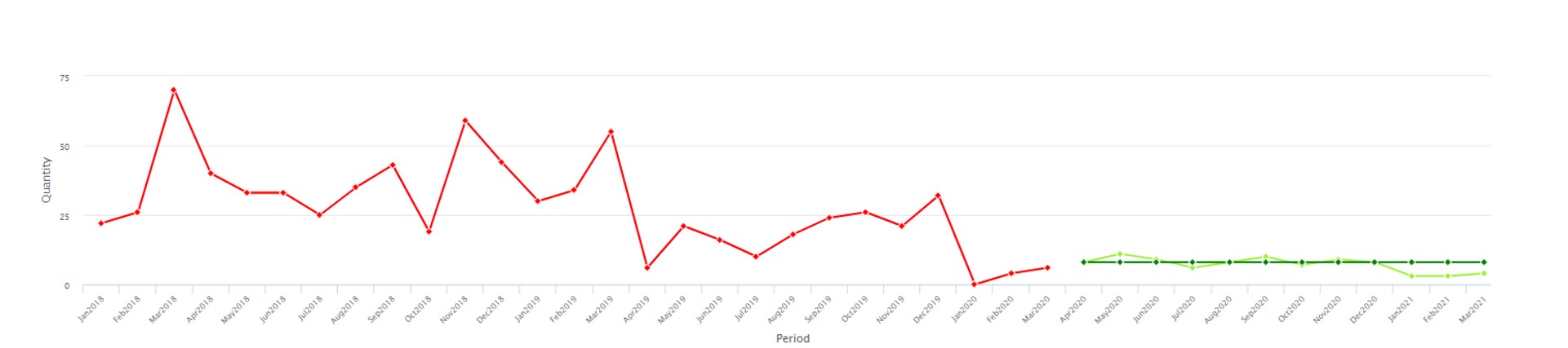
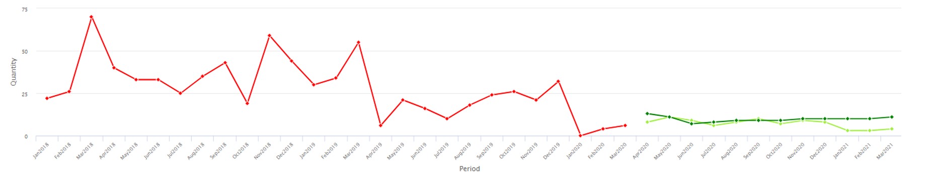
3. Safety stock is inaccurate.  The items being planned for this company are spare parts to support diagnostic equipment.  The demand on most of these parts is very intermittent and sporadic.  So, the choice of using an average to compute lead time demand wasn’t unreasonable if you accept the need for ignoring variability in lead times.  However, the reliance on a Normal distribution to determine the safety stock was a big mistake that resulted in inaccurate safety stocks.  The company stated that its service levels for long lead time items ran in the 90% range compared to their target of 97.7%, and that they made up the difference with expedites.  Achieved service levels for shorter lead time items were about 80%, despite being targeted for 88.4%.    They computed safety stock incorrectly because their demand isn’t “bell shaped” yet they picked safety stocks assuming they were.  This simplification results in missing service level targets, forcing the manual review of many items that then need to be manually “monitored for several periods” by a planner.  Wouldn’t it be better to make sure the reorder point met the exact service level you wanted from the start?  This would ensure you hit your service levels while minimizing unneeded manual intervention.

There is a fourth issue that didn’t make the list but is worth mentioning.  The spreadsheet was unable to track trend or seasonal patterns.  Historical averages ignore trend and seasonality, so the cumulative demand over lead time used in the ROP will be substantially less accurate for trending or seasonal parts. The planning team acknowledged this but didn’t feel it was a legitimate issue, reasoning that most of the demand was intermittent and didn’t have seasonality.  It is important for the model to pick up on trend and seasonality on intermittent data if it exists, but we didn’t find their data exhibited these patterns.  So, we agreed that this wasn’t an issue for them.  But as planning tempo increases to the point that demand is bucketed daily, even intermittent demand very often turns out to have day-of-week and sometimes week-of-month seasonality. If you don’t run at a higher frequency now, be aware that you may be forced to do so soon to keep up with more agile competition. At that point, spreadsheet-based processing will just not be able to keep up.

In conclusion, don’t use spreadsheets. They are not conducive to meaningful what-if analyses, they are too labor-intensive, and the underlying logic must be dumbed down to process quickly enough to be useful.  In short, go with purpose-built solutions. And make sure they run in the cloud.

Smart IP&O is powered by the SmartForecasts® forecasting engine that automatically selects the most appropriate method for each item.  Smart Forecast methods are listed below:

• Simple Moving Average and Single Exponential Smoothing for flat, noisy data
• Linear Moving Average and Double Exponential Smoothing for trending data
• Winters Additive and Winters Multiplicative for seasonal and seasonal & trending data.

This blog explains how each model works using time plots of historical and forecast data.  It outlines how to go about choosing which model to use.   The examples below show the same history, in red, forecasted with each method, in dark green, compared to the Smart-chosen winning method, in light green.

Seasonality
If you want to force (or prevent) seasonality to show in the forecast, then choose Winters models.  Both methods require 2 full years of history.

`Winter’s multiplicative will determine the size of the peaks or valleys of seasonal effects based on a percentage difference from a trending average volume.  It is not a good fit for very low volume items due to division by zero when determining that percentage. Note in the image below that the large percentage drop in seasonal demand in the history is being projected to continue over the forecast horizon making it look like there isn’t any seasonal demand despite using a seasonal method.

Statistical forecast produced with Winter’s multiplicative method. 

Winter’s additive will determine the size of the peaks or valleys of seasonal effects based on a unit difference from the average volume.  It is not a good fit if there’s significant trend to the data.  Note in the image below that seasonality is now being forecasted based on the average unit change in seasonality. So, the forecast still clearly reflects the seasonal pattern despite the down trend in both the level and seasonal peaks/valleys.

Statistical forecast produced with Winter’s additive method.

Trend

If you want to force (or prevent) trend up or down to show in the forecast, then restrict the chosen methods to (or remove the methods of) Linear Moving Average and Double Exponential Smoothing.

 Double exponential smoothing will pick up on a long-term trend.  It is not a good fit if there are few historical data points.

Statistical forecast produced with Double Exponential Smoothing

Linear moving average will pick up on nearer term trends.  It is not a good fit for highly volatile data

Non-Trending and Non-Seasonal Data
If you want to force (or prevent) an average from showing in the forecast, then restrict the chosen methods to (or remove the methods of) Simple Moving Average and Single Exponential Smoothing.

Single exponential smoothing will weigh the most recent data more heavily and produce a flat-line forecast.  It is not a good fit for trending or seasonal data.

Statistical forecast using Single Exponential Smoothing

Simple moving average will find an average for each period, sometimes appearing to wiggle, and better for longer-term averaging.  It is not a good fit for trending or seasonal data.

Statistical forecast using Simple Moving Average

The best inventory planning processes rely on statistical analysis to uncover relevant facts about the data. For instance:

1. The range of demand values and supplier lead times to expect.
2. The most likely values of item demand and supplier lead time.
3. The full probability distributions of item demand and supplier lead time.

If you reach the third level, you have the facts required to answer important operational questions, additional questions such as:

1. Exactly how much extra stock is needed to improve service levels by 5%?
2. What will happen to on-time-delivery if inventory is reduced by 5%?
3. Will either of the above changes generate a positive financial return?
4. More generally, what service level target and associated inventory level is most profitable?

When you have the facts and add your business knowledge, you can make more informed stocking decisions that will generate significant returns. You’ll also set proper expectations with internal and external stakeholders, ensuring there are fewer unwelcome surprises.

Sometimes a statistical forecast just doesn’t make sense.  Every forecaster has been there.  They may double-check that the data was input correctly or review the model settings but are still left scratching their head over why the forecast looks very unlike the demand history.   When the occasional forecast doesn’t make sense, it can erode confidence in the entire statistical forecasting process.

This blog will help a layman understand what the Smart statistical models are and how they are chosen automatically.  It will address how that choice sometimes fails, how you can know if it did, and what you can do to ensure that the forecasts can always be justified.  It’s important to know to expect, and how to catch the exceptions so you can rely on your forecasting system.

How methods are chosen automatically

The criteria to automatically choose one statistical method out of a set is based on which method came closest to correctly predicting held-out history.  Earlier history is passed to each method and the result is compared to actuals to find the one that came closest overall.  That automatically chosen method is then fed all the history to produce the forecast. Check out this blog to learn more about the model selection https://smartcorp.com/uncategorized/statistical-forecasting-how-automatic-method-selection-works/

For most time series, this process can capture trends, seasonality, and average volume accurately. But sometimes a chosen method comes mathematically closest to predicting the held-out history but doesn’t project it forward in a way that makes sense.  That means the system selected method isn’t best and for some “hard to forecast”

Hard to forecast items

Hard to forecast items may have large, unpredictable spikes in demand, or typically no demand but random irregular blips, or unusual recent activity.  Noise in the data sometimes randomly wanders up or down, and the automated best-pick method might forecast a runaway trend or a grind into zero.  It will do worse than common sense and in a small percentage of any reasonably varied group of items.  So, you will need to identify these cases and respond by overriding the forecast or changing the forecast inputs.

How to find the exceptions

Best practice is to filter or sort the forecasted items to identify those where the sum of the forecast over the next year is significantly different than the corresponding history last year.  The forecast sum may be much lower than the history or vice versa.  Use supplied metrics to identify these items; then you can choose to apply overrides to the forecast or modify the forecast settings.

How to fix the exceptions

Often when the forecast seems odd, an averaging method, like Single Exponential Smoothing or even a simple average using Freestyle, will produce a more reasonable forecast.  If trend is possibly valid, you can remove only seasonal methods to avoid a falsely seasonal result.  Or do the opposite and use only seasonal methods if seasonality is expected but wasn’t projected in the default forecast.  You can use the what-if features to create any number of forecasts, evaluate & compare, and continue to fine tune the settings until you are comfortable with the forecast.

Cleaning the history, with or without changing the automatic method selection, is also effective at producing reasonable forecasts. You can embed forecast parameters to reduce the amount of history used to forecast those items or the number of periods passed into the algorithm so earlier, outdated history is no longer considered.  You can edit spikes or drops in the demand history that are known anomalies so they don’t influence the outcome.  You can also work with the Smart team to implement automatic outlier detection and removal so that data prior to being forecasted is already cleansed of these anomalies.

If the demand is truly intermittent, it is going to be nearly impossible to forecast “accurately” per period. If a level-loading average is not acceptable, handling the item by setting inventory policy with a lead time forecast can be effective.  Alternatively, you may choose to use “same as last year” models which while not prone to accuracy will be generally accepted by the business given the alternatives forecasts.

Finally, if the item was introduced so recently that the algorithms do not have enough input to accurately forecast, a simple average or manual forecast may be best.  You can identify new items by filtering on the number of historical periods.

Manual selection of methods

Once you have identified rows where the forecast doesn’t make sense to the human eye, you can choose a smaller subset of all methods to allow into the forecast run and compare to history.  Smart will allow you to use a restricted set of methods just for one forecast run or embed the restricted set to use for all forecast runs going forward. Different methods will project the history into the future in different ways.  Having a sense of how each works will help you choose which to allow.

Rely on your forecasting tool

The more you use Smart period over period to embed your decisions about how to forecast and what historical data to consider, the less often you will face exceptions as described in this blog.  Entering forecast parameters is a manageable task when starting with critical or high impact items.  Even if you don’t embed any manual decisions on forecast methods, the forecast re-runs every period with new data. So, an item with an odd result today can become easily forecastable in time.

When managing service parts, you don’t know what will break and when because part failures are random and sudden. As a result, demand patterns are most often extremely intermittent and lack significant trend or seasonal structure. The number of part-by-location combinations is often in the hundreds of thousands, so it’s not feasible to manually review demand for individual parts. Nevertheless, it is much more straightforward to implement a planning and forecasting system to support spare parts planning than you might think.

This conclusion is informed by hundreds of software implementations we’ve directed over the years. Customers managing spare parts and service parts (the latter for internal consumption/MRO), and to a lesser degree aftermarket parts (for resale to installed bases), have consistently implemented our parts planning software faster than their peers in manufacturing and distribution.

The primary reason is the role in manufacturing and distribution of business knowledge about what might happen in the future. In a traditional B2B manufacturing and distribution environment, there are customers and sales and marketing teams selling to those customers. There are sales goals, revenue expectations, and budgets. This means there is a lot of business knowledge about what will be purchased, what will be promoted, whose opinions need to be accounted for. A complex planning loop is required. In contrast, when managing spare parts, you have a maintenance team that fixes equipment when it breaks. Though there are often maintenance schedules for guidance, what is needed beyond a standard list of consumable parts is often unknown until a maintenance person is on-site. In other words, there just isn’t the same sort of business knowledge available to parts planners when making stocking decisions.

Yes, that is a disadvantage, but it also has an upside: there is no need to produce a period-by-period consensus demand forecast with all the work that requires. When planning spare parts, you can usually skip many steps required for a typical manufacturer, distributor, or retailer. These skippable steps include:  

1. Building forecasts at different levels of the business, such as product family or region.
2. Sharing the demand forecast with sales, marketing, and customers.
3. Reviewing forecast overrides from sales, marketing, and customers.
4. Agreeing on a consensus forecast that combines statistics and business knowledge.
5. Measuring “forecast value add” to determine if overrides make the forecast more accurate.
6. Adjusting the demand forecast for known future promotions.
7. Accounting for cannibalization (i.e., if I sell more of product A, I’ll sell less of product B).

Freed from a consensus-building process, spare parts planners and inventory managers can rely directly on their software to predict usage and the required stocking policies. If they have access to a field-proven solution that addresses intermittent demand, they can quickly “go live” with more accurate demand forecasts and estimates of reorder points, safety stocks, and order suggestions.  Their attention can be focused on getting accurate usage and supplier lead time data. The “political” part of the job can be limited to obtaining organization consensus on service level targets and inventory budgets.

​