Is safety stock regarded as emergency spares or as a day-to-day buffer against spikes in demand? Knowing the difference and configuring your ERP properly will make a big difference to your bottom line.

The Safety Stock field in your ERP system can mean very different things depending on the configuration. Not understanding these differences and how they impact your bottom line is a common issue we’ve seen arise in implementations of our software.

Implementing inventory optimization software starts with new customers completing the technical implementation to get data flowing.  They then receive user training and spend weeks carefully configuring their initial safety stocks, reorder levels, and consensus demand forecasts with Smart IP&O.  The team becomes comfortable with Smart’s key performance predictions (KPPs) for service levels, ordering costs, and inventory on hand, all of which are forecasted using the new stocking policies.

But when they save the policies and forecasts to their ERP test system, sometimes the orders being suggested are far larger and more frequent than they expected, driving up projected inventory costs.

When this happens, the primary culprit is how the ERP is configured to treat safety stock.  Being aware of these configuration settings will help planning teams better set expectations and achieve the expected outcomes with less effort (and cause for alarm!).

Here are the three common examples of ERP safety stock configurations:

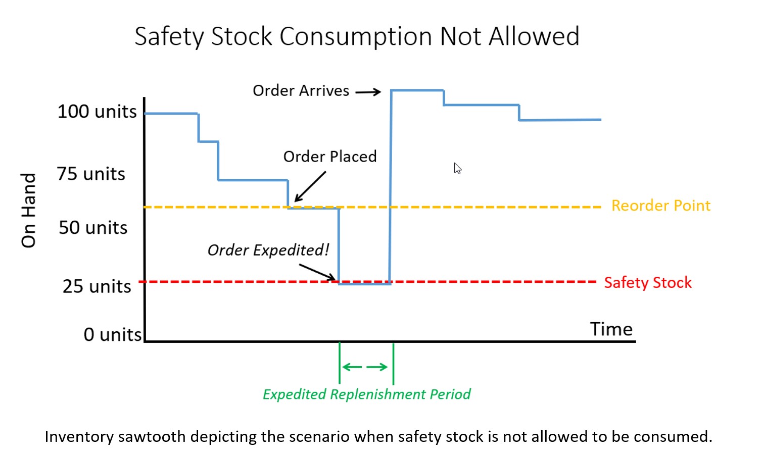
Configuration 1. Safety Stock is treated as emergency stock that can’t be consumed. If a breach of safety stock is predicted, the ERP system will force an expedite no matter the cost so the inventory on hand never falls below safety stock, even if a scheduled receipt is already on order and scheduled to arrive soon.

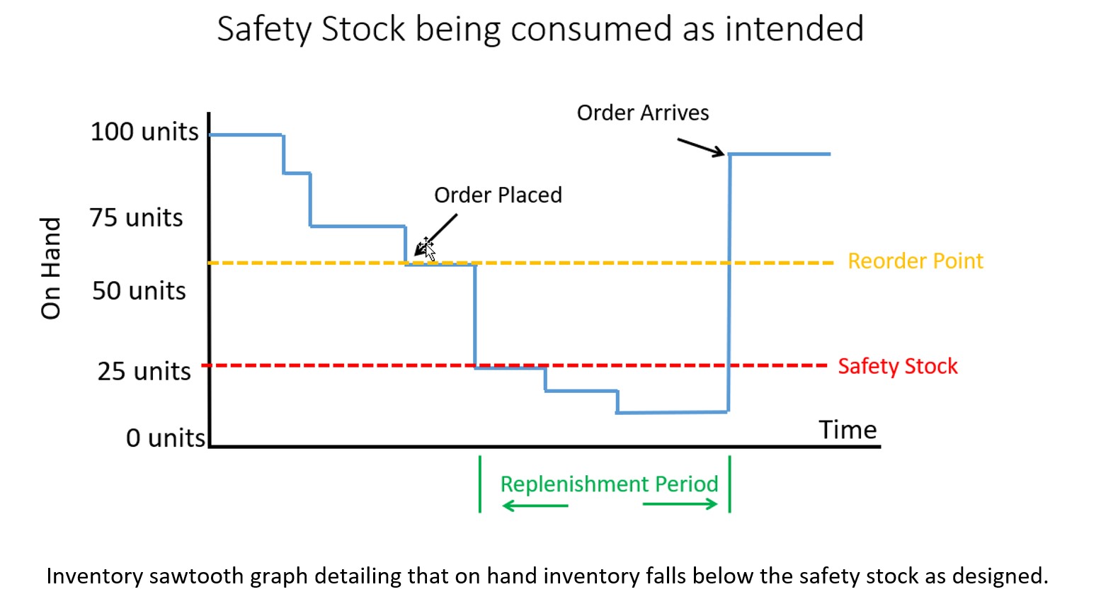
Configuration 2. Safety Stock is treated as Buffer stock that is designed to be consumed. The ERP system will place an order when a breach of safety stock is predicted but on hand inventory will be allowed to fall below the safety stock. The buffer stock protects against stockout during the resupply period (i.e., the lead time).

Configuration 3. Safety Stock is ignored by the system and treated as a visual planning aid or rule of thumb. It is ignored by supply planning calculations but used by the planner to help make manual assessments of when to order.

Note: We never recommend using the safety stock field as described in Configuration 3. In most cases, these configurations were not intended but result from years of improvisation that have led to using the ERP in a non-standard way.  Generally, these fields were designed to programmatically influence the replenishment calculations.  So, the focus of our conversation will be on Configurations 1 and 2. 

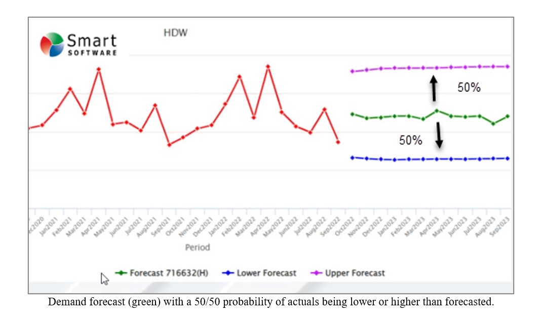
Forecasting and inventory optimization systems are designed to compute forecasts that will anticipate inventory draw down and then calculate safety stocks sufficient to protect against variability in demand and supply. This means that the safety stock is intended to be used as a protective buffer (Configuration 2) and not as emergency sparse (Configuration 3).  It is also important to understand that, by design, the safety stock will be consumed approximately 50% of the time.

Why 50%? Because actual orders will exceed an unbiased forecast half of the time. See the graphic below illustrating this.  A “good” forecast should yield the value that will come closest to the actual most often so actual demand will either be higher or lower without bias in either direction.

If you configured your ERP system to properly allow consumption of safety stock, then the on hand inventory might look like the graph below.  Note that some safety stock is consumed but avoided a stockout.  The service level you target when computing safety stock will dictate how often you stockout before the replenishment order arrives.  Average inventory is roughly 60 units over the time horizon in this scenario.

If your ERP system is configured to not allow consumption of safety stock and treats the quantity entered in the safety stock field more like emergency spares, then you will have a massive overstock!  Your inventory on hand would look like the graph below with orders being expedited as soon as a breach of safety stock is expected. Average inventory is roughly 90 units, a 50% increase compared to when you allowed safety stock to be consumed.

We often are asked, “Why is the software driving up the inventory?” The answer is that Smart isn’t driving it in either direction – the inputs are driving it, and those inputs are controlled by the users (or admins). Here are four things you can do to get the results you expect.

1. Confirm that your service level targets are commensurate with what you want for that item or group of items. Setting very high targets (95% or more) will likely drive inventory up if you have been coasting along at a lower level and are OK with being there. It’s possible you’ve never achieved the new higher service level but customers have not complained.  Figure out what service level has worked by evaluating historical reports on performance and set your targets accordingly. But keep in mind that competitors may beat you on item availability if you keep using your father’s service level targets.

2. Make sure your understanding of “service level” aligns with the software system’s definition. You may be measuring performance based on how often you ship within one week from receipt of the customer order, whereas the software is targeting reorder points based on your ability to ship right away, not within a week. Clearly the latter will require more inventory to hit the same “service level.” For instance, a 75% same-day service level may correspond to a 90% same-week service level. In this case, you are really comparing apples to oranges. If this is the reason for the excess stock, then determine what “same day” service level is needed to get you to your desired “same week” service level and enter that into the software. Using the less-stringent same-day target will drop the inventory, sometimes very significantly.

3. Evaluate the lead time inputs. We’ve seen instances in which lead times had been inflated to trick old software into producing desired results. Modern software tracks suppliers’ performance by recording their actual lead times over multiple orders, then it takes account of lead time variability in its simulations of daily operations. Watch out if your lead times are fixed at one value that was decided on in the distant past and isn’t current.

4. Check your demand signal. You have lots of historical transactions in your ERP system that can be used in many ways to determine the demand history. If you are using signals such as transfers, or you are not excluding returns, then you may be overstating demand. Spend a little time on defining “demand” in the way that makes most sense for your situation.

Outside of work, you may have heard the famous dictum “Correlation is not causation.” It may sound like a piece of theoretical fluff that, though involved in a recent Noble Prize in economics, isn’t relevant to your work as a demand planner. Is so, you may be only partially correct.

Extrapolative vs Causal Models

Most demand forecasting uses extrapolative models. Also called time-series models, these forecast demand using only the past values of an item’s demand. Plots of past values reveal trend and seasonality and volatility, so there is a lot they are good for. But there is another type of model – causal models —that can potentially improve forecast accuracy beyond what you can get from extrapolative models.

Causal models bring more input data to the forecasting task: information on presumed forecast “drivers” external to the demand history of an item. Examples of potentially useful causal factors include macroeconomic variables like the inflation rate, the rate of GDP growth, and raw material prices. Examples not tied to the national economy include industry-specific growth rates and your own and competitors’ ad spending.  These variables are usually used as inputs to regression models, which are equations with demand as an output and causal variables as inputs.

Forecasting using Causal Models

Many firms have an S&OP process that involves a monthly review of statistical (extrapolative) forecasts in which management adjusts forecasts based on their judgement. Often this is an indirect and subjective way to work causal models into the process without doing the regression modeling.

To actually make a causal regression model, first you have to nominate a list of potentially-useful causal predictor variables. These may come from your subject matter expertise. For example, suppose you manufacture window glass. Much of your glass may end up in new homes and new office buildings. So, the number of new homes and offices being built are plausible predictor variables in a regression equation.

There is a complication here: if you are using the equation to predict something, you must first predict the predictors. For example, sales of glass next quarter may be strongly related to numbers of new homes and new office buildings next quarter. But how many new homes will there be next quarter? That’s its own forecasting problem. So, you have a potentially powerful forecasting model, but you have extra work to do to make it usable.

There is one way to simplify things: if the predictor variables are “lagged” versions of themselves. For example, the number of new building permits issued six months ago may be a good predictor of glass sales next month. You don’t have to predict the building permit data – you just have to look it up.

Is it a causal relationship or just a spurious correlation?

Causal models are the real deal: there is an actual mechanism that relates the predictor variable to the predicted variable. The example of predicting glass sales from building permits is an example.

A correlation relationship is more iffy. There is a statistical association that may or may not provide a solid basis for forecasting. For example, suppose you sell a product that happens to appeal most strongly to Dutch people but you don’t realize this. The Dutch are, on average, the tallest people in Europe. If your sales are increasing and the average height of Europeans is increasing, you might use that relationship to good effect. However, if the proportion of Dutch in the Euro zone is decreasing while the average height is increasing because the mix of men versus women is shifting toward men, what can go wrong? You will expect sales to increase because average height is increasing. But your sales are really mostly to the Dutch, and their relative share of the population is shrinking, so your sales are really going to decrease instead. In this case the association between sales and customer height is a spurious correlation.

How can you tell the difference between true and spurious relationships? The gold standard is to do a rigorous scientific experiment. But you are not likely to be in position to do that. Instead, you have to rely on your personal “mental model” of how your market works. If your hunches are right, then your potential causal models will correlate with demand and causal modeling will pay off for you, either to supplement extrapolative models or to replace them.

We recently met with the IT team at one of our customers to discuss data requirements and installation of our API based integration that would pull data from their on-premises installation of their ERP system.   The IT manager and analyst both expressed significant concern about providing this data and seriously questioned why it needed to be provided at all.  They even voiced concerns that their data might be resold to their competition. Their reaction was a big surprise to us.  We wrote this blog with them in mind and to make it easier for others to communicate why certain data is necessary to support an effective demand planning process. 

Please note that if you are a forecast analyst, demand planner, of supply chain professional then most of what you’ll read below will be obvious.  But what this meeting taught me is that what is obvious to one group of specialists isn’t going to be obvious to another group of specialists in an entirely different field. 

The Four main types of data that are needed are:  

1. Historical transactions, such as sales orders and shipments.
2. Job usage transactions, such as what components are needed to produce finished goods
3. Inventory Transfer transactions, such as what inventory was shipped from one location to another.
4. Pricing, costs, and attributes, such as the unit cost paid to the supplier, the unit price paid by the customer, and various meta data like product family, class, etc.  

Below is a brief explanation of why this data is needed to support a company’s implementation of demand planning software.

Transactional records of historical sales and shipments by customer
Think of what was drawn out of inventory as the “raw material” required by demand planning software.  This can be what was sold to whom and when or what you shipped to whom and when.  Or what raw materials or subassemblies were consumed in work orders and when.  Or what is supplied to a satellite warehouse from a distribution center and when.

The history of these transactions is analyzed by the software and used to produce statistical forecasts that extrapolate observed patterns.  The data is evaluated to uncover patterns such as trend, seasonality, cyclical patterns, and to identify potential outliers that require business attention.  If this data is not generally accessible or updated in irregular intervals, then it is nearly impossible to create a good prediction of the future demand.  Yes, you could use business knowledge or gut feel but that doesn’t scale and nearly always introduces bias into the forecast (i.e., consistently forecasting too high or too low). 

Data is needed at the transactional level to support finer grained forecasting at the weekly or even daily levels.  For example, as a business enters its busy season it may want to start forecasting weekly to better align production to demand.  You can’t easily do that without having the transactional data in a well-structured data warehouse. 

It might also be the case that certain types of transactions shouldn’t be included in demand data.  This can happen when demand results from a steep discount or some other circumstance that the supply chain team knows will skew the results.  If the data is provided in the aggregate, it is much harder to segregate these exceptions.  At Smart Software, we call the process of figuring out which transactions (and associated transactional attributes) should be counted in the demand signal as “demand signal composition.” Having access to all the transactions enables a company to modify their demand signal as needed over time within the software.  Only providing some of the data results in a far more rigid demand composition that can only be remedied with additional implementation work.

Pricing and Costs
The price you sold your products for and the cost you paid to procure them (or raw materials) is critical to being able to forecast in revenue or costs.  An important part of the demand planning process is getting business knowledge from customers and sales teams.  Sales teams tend to think of demand by customer or product category and speak in the language of dollars.  So, it is important to express a forecast in dollars.  The demand planning system cannot do that if the forecast is shown in units only. 

Often, the demand forecast is used to drive or at least influence a larger planning & budgeting process and the key input to a budget is a forecast of revenue.  When demand forecasts are used to support the S&OP process, the Demand Planning software should either average pricing across all transactions or apply “time-phased” conversions that consider the price sold at that time.   Without the raw data on pricing and costs, the demand planning process can still function, but it will be severely impaired. 

Product attributes, Customer Details, and Locations
Product attributes are needed so that forecasters can aggregate forecasts across different product families, groups, commodity codes, etc. It is helpful to know how many units and total projected dollarized demand for different categories.  Often, business knowledge about what the demand might be in the future is not known at the product level but is known at the product family level, customer level, or regional level.  With the addition of product attributes to your demand planning data feed, you can easily “roll up” forecasts from the item level to a family level.  You can convert forecasts at these levels to dollars and better collaborate on how the forecast should be modified.  

Once the knowledge is applied in the form of a forecast override, the software will automatically reconcile the change to all the individual items that comprise the group.  This way, a forecast analyst doesn’t have to individually adjust every part.  They can make a change at the aggregate level and let the demand planning software do the reconciliation for them. 

Grouping for ease of analysis also applies to customer attributes, such as assigned salesperson or a customer’s preferred ship from location.  And location attributes can be useful, such as assigned region.  Sometimes attributes relate to a product and location combination, like preferred supplier or assigned planner, which can differ for the same product depending on warehouse.

A final note on confidentiality

Recall that our customer expressed concern that we might sell their data to a competitor. We would never do that. For decades, we have been using customer data for training purposes and for improving our products. We are scrupulous about safeguarding customer data and anonymizing anything that might be used, for instance, to illustrate a point in a blog post.

“Despite what you’ve seen in your Saturday morning cartoons, elephants can’t jump, and there’s one simple reason: They don’t have to. Most jumpy animals—your kangaroos, monkeys, and frogs—do it primarily to get away from predators.”  — Patrick Monahan, Science.org, Jan 27, 2016.

Now you know why the largest ERP companies can’t develop high quality best-of-breed like solutions. They never had to, so they never evolved to innovate outside of their core focus. 

However, as ERP systems have become commoditized, gaps in their functionality became impossible to ignore. The larger players sought to protect their share of customer wallet by promising to develop innovative add-on applications to fill all the white spaces.  But without that “innovation muscle,” many projects failed, and mountains of technical debt accumulated.

Best-of-breed companies evolved to innovate and have deep functional expertise in specific verticals.  The result is that best of breed ERP add-ons are easier to use, have more features, and deliver more value than the native ERP modules they replace. 

If your ERP provider has already partnered with an innovative best of breed add-on provider*, you’re all set! But if you can only get the basics from your ERP, go with a best-of-breed add-on that has a bespoke integration to the ERP. 

A great place to start your search is to look for ERP demand planning add-ons that add brains to the ERP’s brawn, i.e., those that support inventory optimization and demand forecasting.  Leverage add-on tools like Smart’s statistical forecasting, demand planning, and inventory optimization apps to develop forecasts and stocking policies that are fed back to the ERP system to drive daily ordering. 

*App-stores are a license for the best of breed to sell into the ERP companies base –  being listed  partnerships.