
If you hear the phrase “regime change” on the news, you immediately think of some fraught geopolitical event. Statisticians use the phrase differently, in a way that has high relevance for demand planning and inventory optimization. This blog is about “regime change” in the statistical sense, meaning a major change in the character of the demand for an inventory item.
An item’s demand history is the fuel that powers demand planners’ forecasting machines. In general, the more fuel the better, giving us a better fix on the average level, the volatility, the size and frequency of any spikes, the shape of any seasonality pattern, and the size and direction of any trend.
But there is one big exception to the rule that “more data is better data.” If there is a major shift in your world and new demand doesn’t look like old demand, then old data become dangerous.
Modern software can make accurate forecasts of item demand and suggest wise choices for inventory parameters like reorder points and order quantities. But the validity of these calculations depends on the relevance of the data used in their calculation. Old data from an old regime no longer reflect current reality, so including them in calculations creates forecast error for demand planners and either excess stock or unacceptable stockout rates for inventory planners.
That said, if you were to endure a recent regime change and throw out the obsolete data, you would have a lot less data to work with. This has its own costs, because all the estimates computed from the data would have greater statistical uncertainty even though they would be less biased. In this case, your calculations would have to rely more heavily on a blend of statistical analysis and your own expert judgement.
At this point, you may ask “How can I know if and when there has been a regime change?” If you’ve been on the job for a while and are comfortable looking at timeplots of item demand, you will generally recognize regime change when you see it, at least if it’s not too subtle. Figure 1 shows some real-world examples that are obvious.
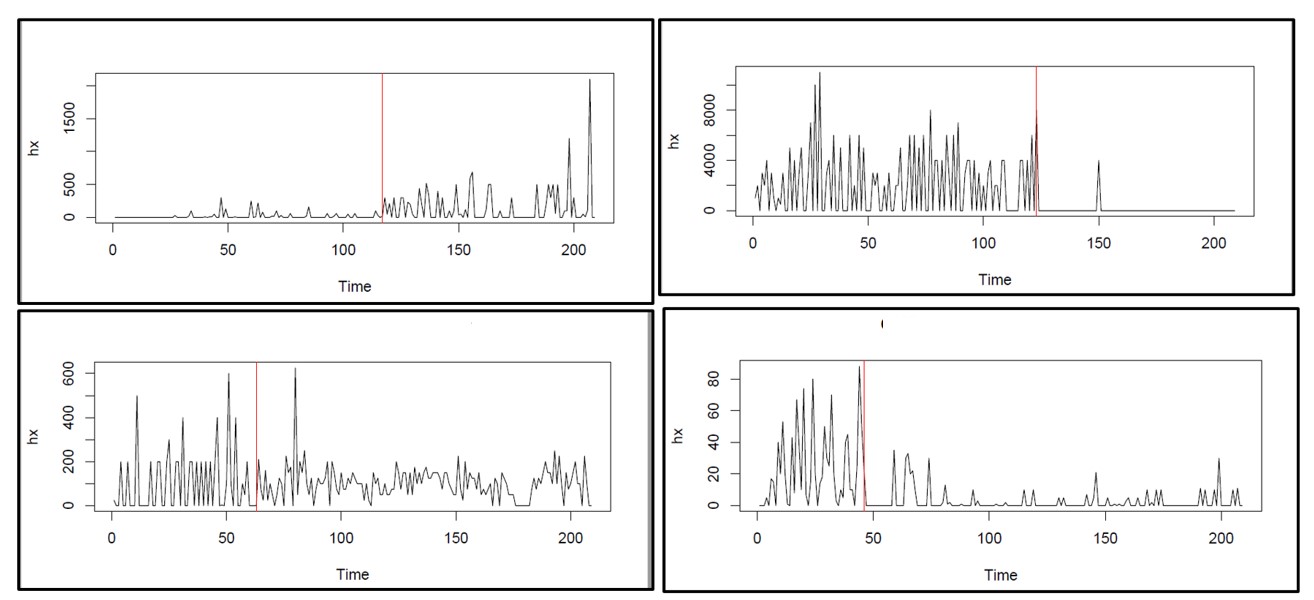
Figure 1: Four examples of regime change in real-world item demand
Unfortunately, less obvious changes can still have significant effects. Moreover, most of our customers are too busy to manually review all the items they manage even once per quarter. When you get beyond, say, 100 items, the task of eyeballing all those time series becomes onerous. Fortunately, software can do a good job of continuously monitoring demand for tens of thousands of items and alerting you to any items that may need your attention. Then too, you can arrange for the software to not only detect regime change but also automatically exclude from its calculations all data collected before the most recent regime change, if any. In other words, you can get both automatic warning of regime change and automatic protection from regime change.
For more on the basics of regime change, see our previous blog on the topic: https://smartcorp.com/blog/demandplanningregimechange/
An Example with Numbers in It
If you would like to learn more, read on to see a numerical example of how much regime change can alter the calculation of a reorder point for a critical spare part. Here is a scenario to illustrate the point.
Scenario
- Goal: calculate the reorder point needed to control the risk of stockout while waiting for replenishment. Assume the target stockout risk is 5%.
- Assume the item has intermittent daily demand, with many days of zero demand.
- Assume daily demand has a Poisson distribution with an average of 1.0 units per day.
- Assume the replenishment lead time is always 30 days.
- The lead time demand will be random, so it will have a probability distribution and the reorder point will be the 95th percentile of the distribution.
- Assume the effect of regime change is to either raise or lower the mean daily demand.
- Assume there is one year of daily data available for estimating the mean daily unit demand.
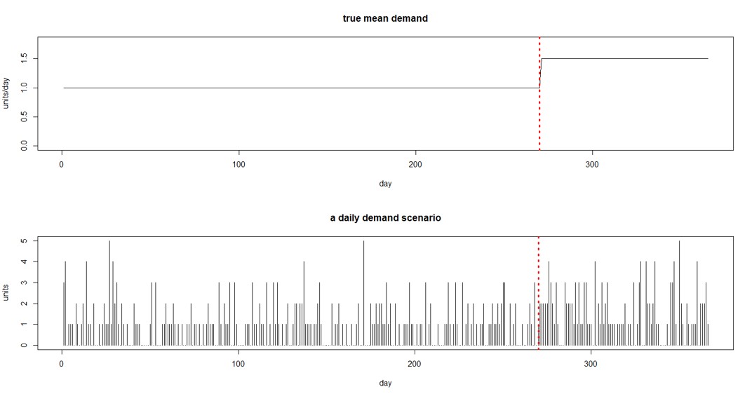
Figure 2 Example of change in mean demand and sample of random daily demand
Figure 2 shows one form of this scenario. The top panel shows that the average daily demand increases from 1.0 to 1.5 after 270 days. The bottom panel shows one way that a year’s worth of daily demand might appear. (At this point, you may be feeling that calculating all this stuff is complicated, even for what turns out to be a simplified scenario. That is why we have software!)
Analysis
Successful calculation of the proper reorder point will depend on when regime change happens and how big a change occurs. We simulated regime changes of various sizes at various times within a 365 day period. Around a base demand of 1.0 units per day, we studied shifts in demand (“shift”) of ±25% and ±50% as well as a no change reference case. We located the time of the change (“t.break”) at 90, 180, and 270 days. In each case, we computed two estimates of the reorder point: The “ideal” value given perfect knowledge of the average demand in the new regime (“ROP.true”), and the estimated value of mean demand computed by ignoring the regime change and using all the demand data for the past year (“ROP.all”).
Table 1 shows the estimates of the reorder point computed over 100 simulations. The center block is the reference case, in which there is no change in the daily demand, which remains fixed at 1 unit per day. The colored block at the bottom is the most extreme increasing scenario, with demand increasing to 1.5 units/day either one-third, one-half, or two-thirds of the way through the year.
We can draw several conclusions from these simulations.
ROP.true: The correct choice for reorder point increases or decreases according to the change in mean demand after the regime change. The relationship is not a simple linear one: the table spans a 600% range of demand levels (0.25 to 1.50) but a 467% range of reorder points (from 12 to 56).
ROP.all: Ignoring the regime change can lead to gross overestimates of the reorder point when demand drops and gross underestimates when demand increases. As we would expect, the later the regime change, the worse the error. For example, if demand increases from 1.0 to 1.5 units per day two-thirds of the way through the year without being noticed, the calculated reorder point of 43 units would fall 13 units short of where it should be.
A word of caution: Table 1 shows that basing the calculations of reorder points using only data from after a regime change will usually get the right answer. What it doesn’t show is that the estimates can be unstable if there is very little demand history after the change. Therefore, in practice, you should wait to react to the regime change until a decent number of observations have accumulated in the new regime. This might mean using all the demand history, both pre- and post-change, until, say, 60 or 90 days of history have accumulated before ignoring pre-change data.
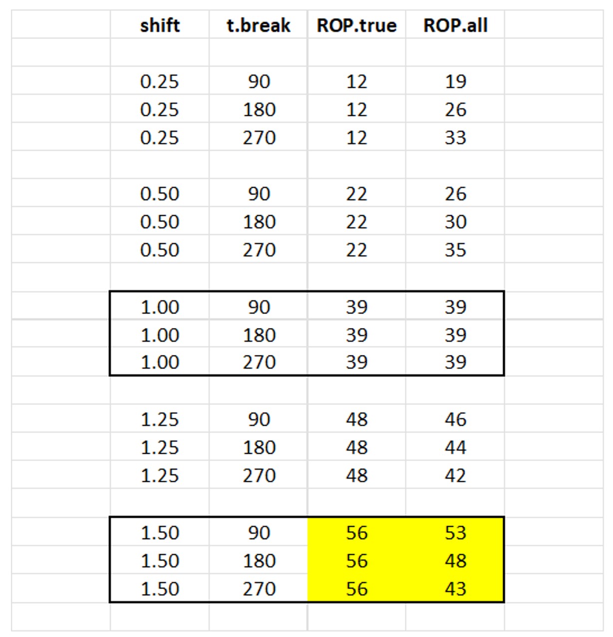
Table 1 Correct and Estimated Reorder Points for different regime change scenarios